An Introduction to Vector Autoregression (VAR)
with tags r var vector autoregression vars -Since the seminal paper of Sims (1980) vector autoregressive models have become a key instrument in macroeconomic research. This post presents the basic concept of VAR analysis and guides through the estimation procedure of a simple model. When I started my undergraduate program in economics I occasionally encountered the abbreviation VAR in some macro papers. I was fascinated by those waves in the boxes titled impulse responses and wondered how difficult it would be to do such reseach on my own. I was motivated, but my first attempts were admittedly embarrassing. It took me quite a long time to figure out which kind of data can be analysed, how to estimate a VAR model and how to obtain meaningful impulse responses. Today, I think that there is nothing fancy about VAR models at all once you keep in mind some points.
Univariate autoregression
VAR stands for vector autoregression. To understand what this means, let us first look at a simple univariate (i.e. only one dependent or endogenous variable) autoregressive (AR) model of the form \(y_{t} = a_1 y_{t-1} + e_t\). In this model the current value of variable \(y\) depends on its own first lag, where \(a_1\) denotes its parameter coefficient and the subscript refers to its lag. Since the model contains only one lagged value the model is called autoregressive of order one, short AR(1), but you can easily increase the order to p by adding more lags, which results in an AR(p). The error term \(e_t\) is assumed to be normally distributed with mean zero and variance \(\sigma^2\).
Stationarity
Before you estimate such a model you should always check if the time series you analyse are stationary, i.e. their means and variances are constant over time and do not show any trending behaviour. This is a very important issue and every good textbook on time series analysis treats it quite – maybe too – intensively. A central problem when you estimate models with non-stationary data is, that you will get improper test statistics, which might lead you to choose the wrong model.
There is a series of statistical tests like the Dickey-Fuller, KPSS, or the Phillips-Perron test to check whether a series is stationary. Another very common practise is to plot a series and check if it moves around a constant mean value, i.e. a horizontal line. If this is the case, it is likely to be stationary. Both statistical and visual tests have their drawbacks and you should always be careful with those approaches, but they are an important part of every time series analysis. Additionally, you might want to check what the economic literature has to say about the stationarity of particular time series like, e.g., GDP, interest rates or inflation. This approach is particularly useful if you want to determine whether a series trend or difference stationary, which must be treated a bit differently.
At this point it should be mentioned that even if two time series are not stationary, a special combination of them can still be stationary. This phenomenon is called cointegration and so-called (vector) error correction models (VECM) can be used to analyse it. For example, this approach can significantly improve the results of an analysis of variables with known equilibrium relationships.
Autoregressive distributed lag models
Regressing a macroeconomic variable solely on its own lags like in an AR(p) model might be a quite restrictive approach. Usually, it is more appropriate to assume that there are further factors that drive a process. This idea is captured by models which contain lagged values of the dependent variable as well as contemporaneous and lagged values of other, i.e. exogenous, variables. Again, these exogenous variables should be stationary. For an endogenous variable \(y_{t}\) and an exogenous variable \(x_{t}\) such an autoregressive distributed lag, or ADL, model can be written as
\[y_{t} = a_1 y_{t-1} + b_0 x_{t}+ b_{1} x_{t-1} + e_t.\]
In this ADL(1,1) model \(a_1\) and \(e_t\) are definded as above and \(b_0\) and \(b_1\) are the coefficients of the contemporaneous and lagged value of the exogenous variable, respectively.
The forecasting performance of such an ADL model is likely to be better than for a simple AR model. However, what if the exogenous variable depends on lagged values of the endogenous variable too? This would mean that \(x_{t}\) is endogenous too and there is further space to improve our forecasts.
Vector autoregressive models
At this point the VAR approach comes in. A simple VAR model can be written as
\[\begin{pmatrix} y_{1t} \\ y_{2t} \end{pmatrix} = \begin{bmatrix} a_{11} & a_{12} \\ a_{21} & a_{22} \end{bmatrix} \begin{pmatrix} y_{1t-1} \\ y_{2t-1} \end{pmatrix} + \begin{pmatrix} \epsilon_{1t} \\ \epsilon_{2t} \end{pmatrix}\]
or, more compactly,
\[ y_t = A_1 y_{t-1} + \epsilon_t,\] where \(y_t = \begin{pmatrix} y_{1t} \\ y_{2t} \end{pmatrix}\), \(A_1= \begin{bmatrix} a_{11} & a_{12} \\ a_{21} & a_{22} \end{bmatrix}\) and \(\epsilon_t = \begin{pmatrix} \epsilon_{1t} \\ \epsilon_{2t} \end{pmatrix}.\)
Note: Yes, you should familiarise yourself with some (basic) matrix algebra (addition, subtraction, multiplication, transposition, inversion and the determinant), if you want to work with VARs.
Basically, such a model implies that everything depends on everything. But as can be seen from this formulation, each row can be written as a separate equation, so that \(y_{1t} = a_{11} y_{1t-1} + a_{12} y_{2t-1} + \epsilon_{1t}\) and \(y_{2t} = a_{21} y_{1t-1} + a_{22} y_{2t-1} + \epsilon_{2t}\). Hence, the VAR model can be rewritten as a series of individual ADL models as described above. In fact, it is possible to estimate VAR models by estimating each equation separately.
Looking a bit closer at the single equations you will notice, that there appear no contemporaneous values on the right-hand side (rhs) of the VAR model. However, information about contemporaneous relations can be found in the so-called variance-covariance matrix \(\Sigma\). It contains the variances of the endogenous variable on its diagonal elements and covariances of the errors on the off-diagonal elements. The covariances contain information about contemporaneous effects between the variables. Like the error variance \(\sigma^2\) in a single equation model \(\Sigma\) is essential for the calculation of test statistics and confidence intervals.
The covariance matrices of standard VAR models are symmetric, i.e. the elements to the top-right of the diagonal (the “upper triangular”) mirror the elements to the bottom-left of the diagonal (the “lower triangular”). This reflects the idea that the relations between the endogenous variables only reflect correlations and do not allow to make statements about causal relationships, since the effects are the same in each direction. This is the reason why this model is said to be not uniquely identified.
Contemporaneous causality or, more precisely, the structural relationships between the variables is analysed in the context of so-called structural VAR (SVAR) models, which impose special restrictions on the covariance matrix – and depending on the model on other matrices as well – so that the system is identified. This means that there is only one unique solution for the model and it is clear, how the causalities work. The drawback of this approach is that it depends on the more or less subjective assumptions made by the researcher.1 For many researchers this is too much subjectiv information, even if sound economic theory is used to justify those assumptions.
In this article I consider a VAR(2) process of the form
\[\begin{pmatrix} y_{1,t}\\ y_{2,t} \end{pmatrix} = \begin{bmatrix} -0.3 & -0.4 \\ 0.6 & 0.5 \end{bmatrix} \begin{pmatrix} y_{1,t-1} \\ y_{2,t-1} \end{pmatrix} + \begin{bmatrix} -0.1 & 0.1 \\ -0.2 & 0.05 \end{bmatrix} \begin{pmatrix} y_{1,t-2} \\ y_{2,t-2} \end{pmatrix} + \begin{pmatrix} \epsilon_{1t} \\ \epsilon_{2t} \end{pmatrix}\]
with \(\epsilon_{1t} \sim N(0, 0.5)\) and \(\epsilon_{2t} \sim N(0, 0.5)\). Note that for simplification the errors are not correlated. Models with correlated errors are described in a post on SVAR.
The artificial sample for this example is generated in R with
set.seed(123) # Reset random number generator for reasons of reproducability

# Generate sample
t <- 200 # Number of time series observations
k <- 2 # Number of endogenous variables
p <- 2 # Number of lags

# Generate coefficient matrices
A.1 <- matrix(c(-.3, .6, -.4, .5), k) # Coefficient matrix of lag 1
A.2 <- matrix(c(-.1, -.2, .1, .05), k) # Coefficient matrix of lag 2
A <- cbind(A.1, A.2) # Companion form of the coefficient matrices

# Generate series
series <- matrix(0, k, t + 2*p) # Raw series with zeros
for (i in (p + 1):(t + 2*p)){ # Generate series with e ~ N(0,0.5)
  series[, i] <- A.1%*%series[, i-1] + A.2%*%series[, i-2] + rnorm(k, 0, .5)
}

series <- ts(t(series[, -(1:p)])) # Convert to time series format
names <- c("V1", "V2") # Rename variables

plot.ts(series) # Plot the series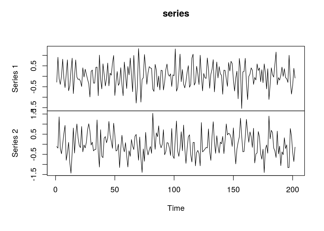
Estimation
The estimation of the parameters and the covariance matrix of a simple VAR model is straightforward. For \(Y = (y_{1},..., y_{T})\) and \(Z = (z_{1},..., z_{T})\) with \(z\) as a vector of lagged valus of \(y\) and possible deterministic terms the least squares estimator of the parameters is \(\hat{A} = YZ(ZZ')^{-1}\). The covariance matrix is then obtained from \(\frac{1}{T-Q}(Y-\hat{A}Z) (Y-\hat{A}Z)'\), where \(Q\) is the number of estimated parameters. These formalas are usually already programmed in standard statistics packages for basic applications.
In order to estimate the VAR model I use the vars package by Pfaff (2008). The relevant function is VAR and its use is straightforward. You just have to load the package and specify the data (y), order (p) and the type of the model. The option type determines whether to include an intercept term, a trend or both in the model. Since the artificial sample does not contain any deterministic term, we neglect it in the estimation by setting type = "none".
library(vars) # Load package

var.1 <- VAR(series, 2, type = "none") # Estimate the model
Model comparison
A central issue in VAR analysis is to find the number of lags, which yields the best results. Model comparison is usually based on information criteria like the AIC, BIC or HQ. Usually, the AIC is preferred over other criteria, due to its favourable small sample forecasting features. The BIC and HQ, however, work well in large samples and have the advantage of being a consistent estimator of the true order, i.e. they prefer the true order of the VAR model - in contrast to the order, which yields the best forecasts - as the sample size grows.
The VAR function of the vars package already allows to calculate standard information criteria to find the best model. In this example we use the AIC:
var.aic <- VAR(series, type = "none", lag.max = 5, ic = "AIC")Note that instead of specifying the order p, we now set the maximum lag length of the model and the information criterion used to select the best model. The function then estimates all five models, compares them according to their AIC values and automatically selects the most favourable. Looking at summary(var.aic) we see that the AIC suggests to use an order of 2 which is the true order.
summary(var.aic)##
## VAR Estimation Results:
## =========================
## Endogenous variables: Series.1, Series.2
## Deterministic variables: none
## Sample size: 200
## Log Likelihood: -266.065
## Roots of the characteristic polynomial:
## 0.6611 0.6611 0.4473 0.03778
## Call:
## VAR(y = series, type = "none", lag.max = 5, ic = "AIC")
##
##
## Estimation results for equation Series.1:
## =========================================
## Series.1 = Series.1.l1 + Series.2.l1 + Series.1.l2 + Series.2.l2
##
## Estimate Std. Error t value Pr(>|t|)
## Series.1.l1 -0.19750 0.06894 -2.865 0.00463 **
## Series.2.l1 -0.32015 0.06601 -4.850 2.51e-06 ***
## Series.1.l2 -0.23210 0.07586 -3.060 0.00252 **
## Series.2.l2 0.04687 0.06478 0.724 0.47018
## ---
## Signif. codes: 0 '***' 0.001 '**' 0.01 '*' 0.05 '.' 0.1 ' ' 1
##
##
## Residual standard error: 0.4638 on 196 degrees of freedom
## Multiple R-Squared: 0.2791, Adjusted R-squared: 0.2644
## F-statistic: 18.97 on 4 and 196 DF, p-value: 3.351e-13
##
##
## Estimation results for equation Series.2:
## =========================================
## Series.2 = Series.1.l1 + Series.2.l1 + Series.1.l2 + Series.2.l2
##
## Estimate Std. Error t value Pr(>|t|)
## Series.1.l1 0.67381 0.07314 9.213 < 2e-16 ***
## Series.2.l1 0.34136 0.07004 4.874 2.25e-06 ***
## Series.1.l2 -0.18430 0.08048 -2.290 0.0231 *
## Series.2.l2 0.06903 0.06873 1.004 0.3164
## ---
## Signif. codes: 0 '***' 0.001 '**' 0.01 '*' 0.05 '.' 0.1 ' ' 1
##
##
## Residual standard error: 0.4921 on 196 degrees of freedom
## Multiple R-Squared: 0.3574, Adjusted R-squared: 0.3443
## F-statistic: 27.26 on 4 and 196 DF, p-value: < 2.2e-16
##
##
##
## Covariance matrix of residuals:
## Series.1 Series.2
## Series.1 0.21417 -0.03116
## Series.2 -0.03116 0.24154
##
## Correlation matrix of residuals:
## Series.1 Series.2
## Series.1 1.000 -0.137
## Series.2 -0.137 1.000Looking at the results more closely we can compare the true values - cointained in object A - with the parameter estimates of the model:
# True values
A
## [,1] [,2] [,3] [,4]
## [1,] -0.3 -0.4 -0.1 0.10
## [2,] 0.6 0.5 -0.2 0.05# Extract coefficients, standard errors etc. from the object
# produced by the VAR function
est_coefs <- coef(var.aic)
# Extract only the coefficients for both dependend variables
# and combine them to a single matrix
est_coefs <- rbind(est_coefs[[1]][, 1], est_coefs[[2]][, 1])
# Print the rounded estimates in the console
round(est_coefs, 2)## Series.1.l1 Series.2.l1 Series.1.l2 Series.2.l2
## [1,] -0.20 -0.32 -0.23 0.05
## [2,] 0.67 0.34 -0.18 0.07All the estimates have the right sign and are relatively close to their true values. I leave it to you to look at the standard errors of summary(var.aic) to check whether the true values fall into the confidence bands of the estimates.
Impulse response
Once we have decided on a final VAR model its estimated parameter values have to be interpreted. Since all variables in a VAR model depend on each other, individual parameter values only provide limited information on the reaction of the system to a shock. In order to get a better intuition of the model’s dynamic behaviour, impulse responses (IR) are used. They give the reaction of a response variable to a one-time shock in an impulse variable. The trajectory of the response variable can be plotted, which results in those wavy curves that can be found in many macro papers.
In R the irf function of the vars package can be used to obtain an impulse response function. In the following example, we want to know how Series 2 behaves after a shock to Series 1. After specifying the model and the variables for which we want an impulse response we set the time horizon n.ahead to 20. The plot gives the response of series 2 for the periods 0 to 20 to a shock in series 1 in period 0. The function also automatically calculates so-called bootstrap confidence bands. (Bootstrapping is a common procedure in impulse response analysis. But you should keep in mind that it has its drawbacks when you work with structural VAR models though.)
# Calculate the IRF
ir.1 <- irf(var.1, impulse = "Series.1", response = "Series.2", n.ahead = 20, ortho = FALSE)

# Plot the IRF
plot(ir.1)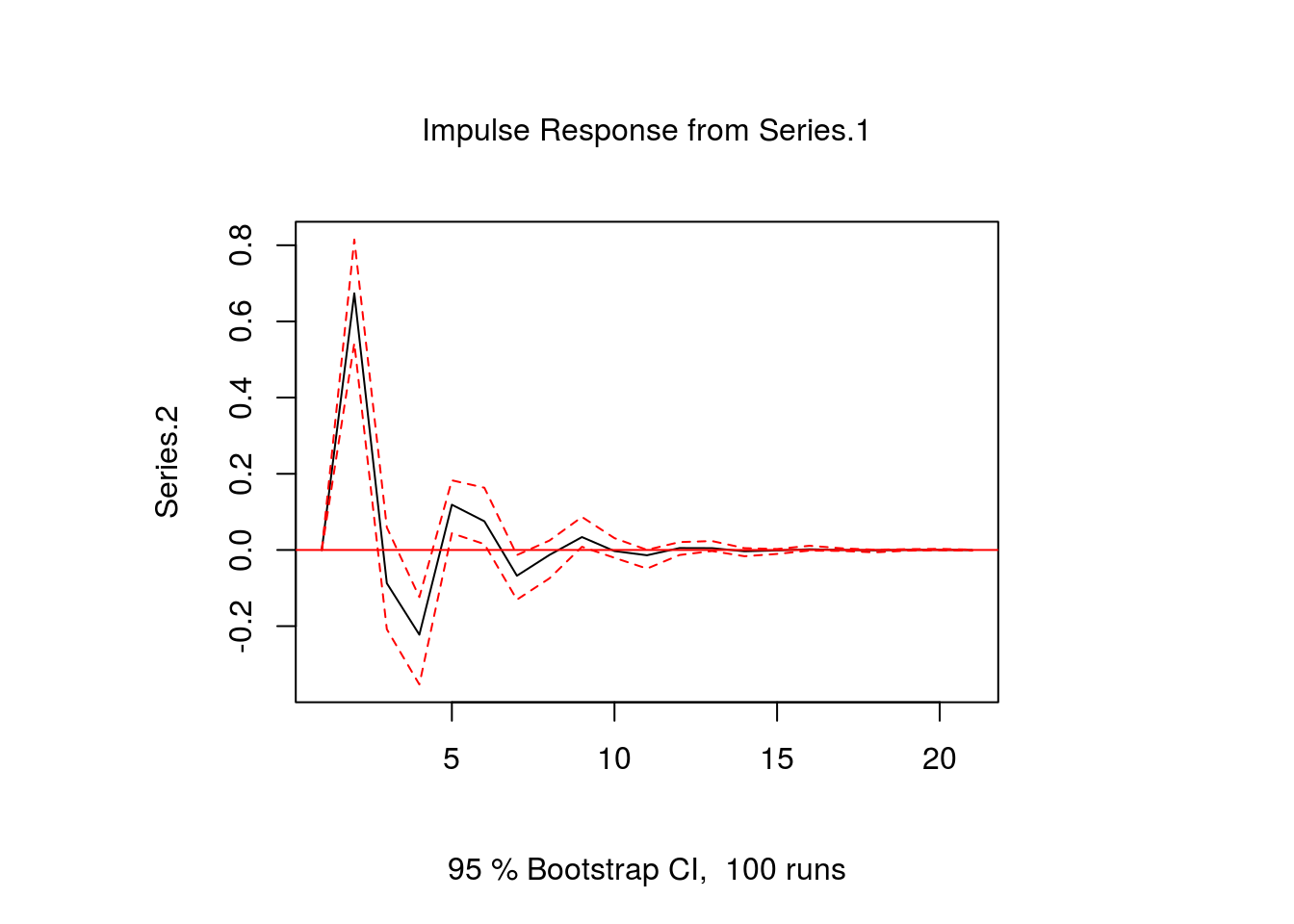
Note that the ortho option is important, because it says something about the contemporaneous relationships between the variables. In our example we already know that such relationships do not exist, because the true variance-covariance matrix – or simply covariance matrix – is diagonal with zeros in the off-diagonal elements. However, since the limited time series data with 200 observations restricts the precision of the parameter estimates, the covariance matrix has positive values in its off-diagonal elements which implies non-zero contemporaneous effects of a shock. To rule this out in the IR, we set ortho = FALSE. The result of this is that the impulse response starts at zero in period 0. You could also try out the alternative and set ortho = TRUE, which results in a plot that start below zero. I do not want to go into more detail here, but suffice it so say that the issue of so-called orthogonal errors is one of the central problems in VAR analysis and you should definitely read more about it, if you plan to set up your own VAR models.
Sometimes it is interesting to see what the long-run effects of a shock are. To get an idea about that you can also calculate and plot the cumulative impulse response function to get an idea of the overall long-run effect of the shock:
# Calculate impulse response
ir.2 <- irf(var.1,impulse="Series.1",response="Series.2",n.ahead = 20,ortho = FALSE,
cumulative = TRUE)

# Plot
plot(ir.2)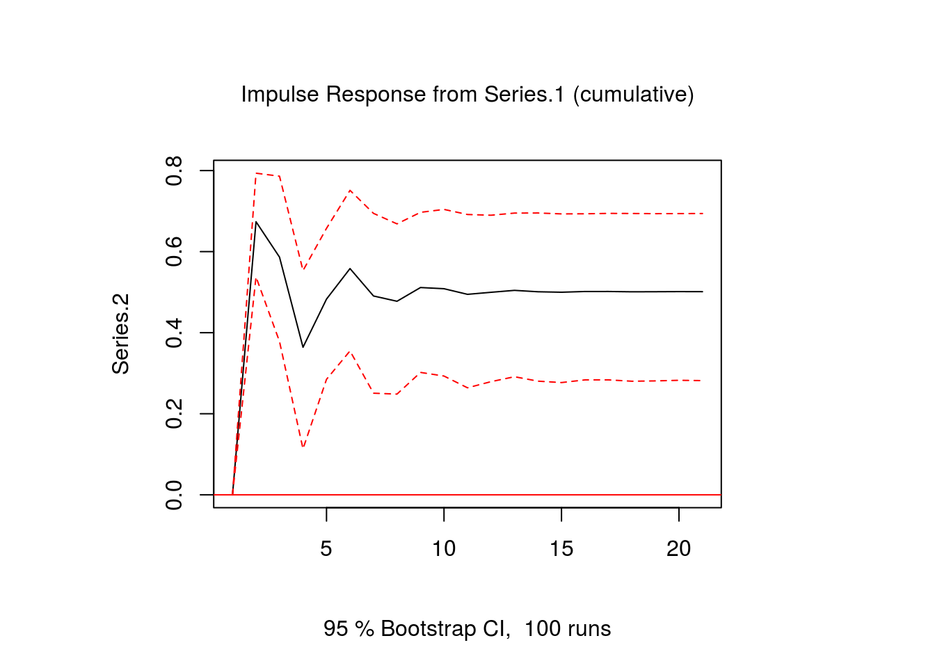
We see that although the reaction of series 2 to a shock in series 1 is negative during some periods, the overall effect significantly positive.
References
Lütkepohl, H. (2007). New Introduction to Multiple Time Series Analyis. Berlin: Springer.
Bernhard Pfaff (2008). VAR, SVAR and SVEC Models: Implementation Within R Package vars. Journal of Statistical Software 27(4).
Sims, C. (1980). Macroeconomics and Reality. Econometrica, 48(1), 1–48.
If you want to impress your professor, you can also use the term Wold-ordering problem to refer to this issue.↩