An Introduction to Network Analysis in R
with tags igraph ggraph networks network-analysis -With the increasing availability of granular data on the relationships between individual entities - such as persons (social media), countries (internatinal trade) and financial institutions (supervisory reporting) - network analysis offers many possibilities to extract useful information from such data. This post provides an introduction to network analysis in R using the powerful igraph package for the calculation of metrics and ggraph for visualisation. It marks the beginning of a more comprehensive treatment of network analysis on r-econometrics.
The igraph package
There are multiple packages for the analysis of networks in R. In this post I concentrate on the igraph package, which allows for a broad range of applications. But before we get into it in more detail, it is useful to know that there are two possible ways to represent the edges, i.e. the connections, of a network:
- Adjacency matrix: This is a square matrix, where each row and column corresponds to an entity. If two entities are conencted, the respective field in the matrix takes the value one and zero otherwise.
- A list of connections: In its most simple form this is a list, where each edge of a network is represented by a row with one entity in the first column and the other in the second. For the purpose of this post this is our preferred representation.
Create an artificial graph
We can illustrate these two representations by looking at an artificial network. Such a network could be generated with certain functions of the igraph package. However, the following code only uses base functionalities of R. It results in a data frame with the names of the connected entities in the first and second row. The third row contains a random indicator for the strength of the connection. It is based on the square of a value from a standard normal distribution. To reduce the number of resulting edges, only values above a certain threshold are kept. Also, the code excludes the connections a node has with itself.
# Set seed for reproducibility
set.seed(12345)

# Generate data
raw <- data.frame(byer = rep(letters, 1, each = 26),
                  sllr = rep(letters, 26),
                  con = rnorm(26 * 26)^2) # Calculate arbitrary weights

# Drop connections with oneself
raw <- raw[raw$byer != raw$sllr,]

# Only keep strong connections
raw <- raw[abs(raw$con) > 1,]

# Reformat row numbers
rownames(raw) <- NULL

# Look at result
head(raw)
## byer sllr con
## 1 a f 3.304964
## 2 a l 3.302623
## 3 a s 1.255997
## 4 a v 2.119310
## 5 a x 2.412236
## 6 a y 2.552676Basically, this is a list repesentation of the artifical network. In a next step we convert the data frame to an igraph object.
igraph objects
# Load package
library(igraph)
The transformation is straightforward and can be done with the graph_from_data_frame function, where for simplicity we set the argument directed = FALSE to indicated that the network is not directed. Note that it is important that the first and second column of the data frame contain the names of the nodes that have a connection.
graph_df <- graph_from_data_frame(raw, directed = FALSE)The function simplify can be used to get rid of loops and multiple edges:
graph_df <- simplify(graph_df)Now take a look at the object:
graph_df## IGRAPH bdf5bb9 UN-- 26 173 --
## + attr: name (v/c)
## + edges from bdf5bb9 (vertex names):
## [1] a--f a--g a--l a--m a--s a--v a--x a--y a--z b--d b--f b--g b--h b--k
## [15] b--l b--m b--o b--p b--q b--r b--t b--u b--v b--w b--x b--z c--g c--h
## [29] c--j c--l c--m c--n c--p c--q c--r c--s c--u c--v c--w c--x c--z d--e
## [43] d--f d--h d--o d--q d--t d--x d--z e--f e--g e--h e--i e--j e--k e--o
## [57] e--q e--r e--s e--t e--v e--w e--x e--y e--z f--g f--i f--k f--l f--m
## [71] f--n f--q f--r f--u f--z g--l g--m g--p g--s g--t g--u g--w g--x g--y
## [85] g--z h--m h--o h--r h--s h--t h--v h--x h--y h--z i--j i--k i--n i--q
## [99] i--u i--v i--y i--z j--m j--p j--r j--t j--u j--v j--w j--y j--z k--l
## + ... omitted several edgesIt does not look like the data frame list. However, it can be seen that each element of the list of edges refers to a conenction between to entities.
Let’s compare this list to the adjacency matrix representation. It can be obtained directly from the igraph object by using the as_adj function.
graph_adj <- as_adj(graph_df)Now look at the first six rows and columns of the resulting object.
graph_adj[1:6, 1:6]## 6 x 6 sparse Matrix of class "dgCMatrix"
## a b c d e f
## a . . . . . 1
## b . . . 1 . 1
## c . . . . . .
## d . 1 . . 1 1
## e . . . 1 . 1
## f 1 1 . 1 1 .An existing connection between two nodes is indicated by the value one. If there is no connection between them, the field contains a dot. For example, the (undirected) connection between a and f is described by the 1 in the sixth value of the first column and the sixth value in the first row. This corresponds to the first entry in the list representation of the above igraph object. If the network were directed, only one field would contain a 1 - unless the connection was mutual.
Note that the resulting object is not an object of class igraph. as_adj produces a dgCMatrix object, which comes with the Matrix package and was specifically designed to implement so-called sparse matrices. Sparse matrices are simply matrices which contain a lot of zeros. By only considereing non-zero values, sparse matrices allow for a lot of additional computational efficiency, which is beneficial for the analysis of very large networks.
Summary statistics
This secton covers standard metrics to describe a network. Most of these metrics focus on the centrality of a graph’s nodes. The following desciption is based on Jackson (2008).
Degree
The degree of a node is the number of its connections. The degree function calculates this number for each node of a graph. The node with the highest number is the node with the highest number of connections.
g_degree <- degree(graph_df)

g_degree
## a b c d e f g h i j k l m n o p q r s t u v w x y
## 9 17 15 9 17 14 15 13 10 12 14 10 14 10 14 11 15 16 12 13 14 13 12 16 14
## z
## 17The degree is of a node is an insteresting metric to identify the most connected nodes of a network. However, if the structure of a network is of interest, the degree distribution can be an informative metric. It describes the relative frequencey of nodes that have different degrees. In that way it is a histogram of degrees.
hist(g_degree)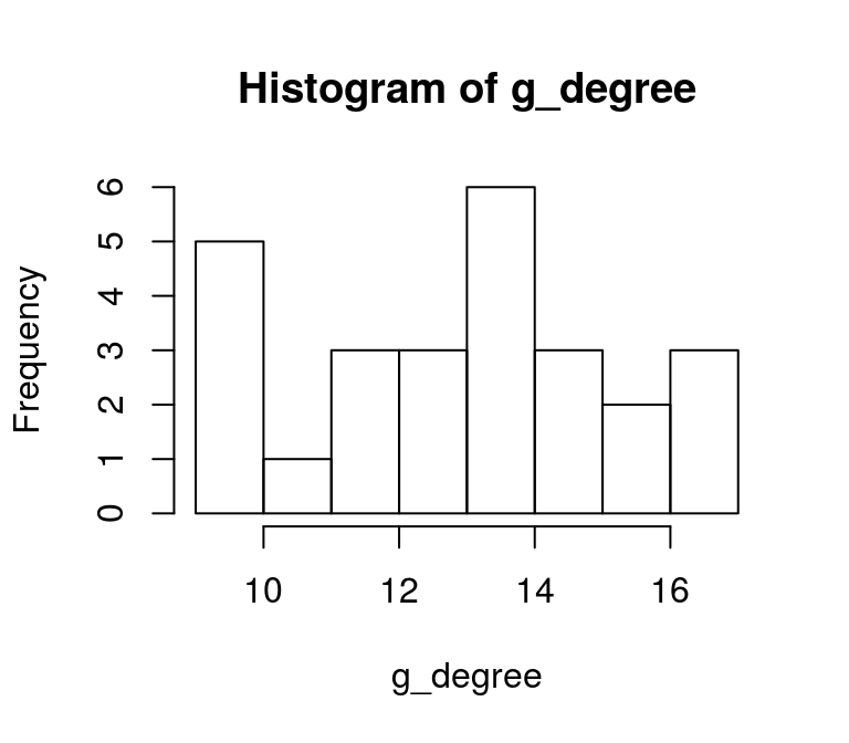
Betweenness
Betweenness denotes the number of shortest paths passing through a node.
g_betw <- betweenness(graph_df)

round(g_betw, 2)
## a b c d e f g h i j k l
## 2.17 9.50 7.79 1.11 10.10 6.85 7.86 4.25 2.19 4.42 6.48 2.12
## m n o p q r s t u v w x
## 5.67 2.93 6.01 3.99 7.56 8.62 3.84 4.53 5.61 6.19 3.15 10.15
## y z
## 7.21 11.68Eigenvector centrality
The eigenvector centrality (Bonabeau, 1972) belongs to the class of spectral centralities. It is based on the idea that the importance of a node is recusively related to the importance of the nodes pointing to it. For example, your popularity depends on the popularity of your friends, whose popularity depends on their friends etc.
g_eigen <- eigen_centrality(graph_df)

round(g_eigen$vector, 2)
## a b c d e f g h i j k l m n o
## 0.54 1.00 0.87 0.58 0.99 0.81 0.88 0.81 0.60 0.72 0.82 0.61 0.85 0.61 0.84
## p q r s t u v w x y z
## 0.64 0.89 0.94 0.72 0.79 0.85 0.76 0.73 0.92 0.80 0.97Further measures will be added in the future.
Visualisation
Beside the calculation of summarising network metrics, the visualisation of a graph can also be a very informative step in network analysis. Since visualisations in R usually involve the ggplot2 package, I focus on the ggraph package, which is based on the ggplot2 architecture. However, the plot function can be used to get a quick impression of a network:
plot(graph_df)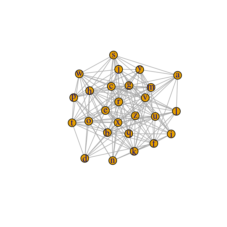
When using ggplot2 the main challenge in the visualisation of networks is to find suitable x- and y-coordinates for the nodes of a graph. Fortunately, there are some packages out there, which were developed for this purpose. For example, ggraph and ggnetwork take an igraph object and produce tables with suitable coordianates. These coordinates are usually obtained by using special algorithms such as the ones proposed by Fruchterman and Reingold (1991) or Kamada and Kawai (1989). The latter is applied in the code below.
ggraph diagrams follow the ggplot2 logic, where the function ggplot is replaced by ggraph to set up the graph. The function is then followed by the layers the user wants to add. In this example we add a layer of edges with geom_edge_link and on top of this a layer of nodes, which are represented by points, using geom_node_point.
# Load packages
library(ggraph)
library(ggplot2)

ggraph(graph_df, layout = "kk") + # Generate graph
  geom_edge_link(colour = "darkgrey") + # Add a layer of edges
  geom_node_point(size = 3) + # Add a layer of nodes
  theme_graph() # Get rid of gray background colour, grid and axes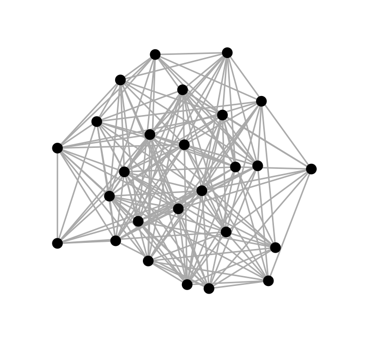
Further introductions to ggraph can be found on https://www.data-imaginist.com/tags/ggraph and in the package’s vignettes, of course.
References
Bonabeau, E. (1972). Factoring and weighting approaches to status scores and clique identification. Journal of Mathematical Sociology 2, 113-120.
Csardi G., & Nepusz, T. (2006). The igraph software package for complex network research, InterJournal Complex Systems, 1695.
Fruchterman, T. M. J., & Reingold, E. M. (1991). Graph Drawing by Force-directed Placement. Software - Practice and Experience, 21(11), 1129-1164.
Jackson, M. O. (2008). Social and economic networks. Princeton: University Press.
Kamada, T., & Kawai, S. (1989). An algorithm for drawing general undirected graphs. Information Processing Letters 31(1), 7-15.