Decomposing Inflation for EA Countries
As a result of supply chain disruptions due to the Covid-19 pandemic and the recent war in the Ukraine inflation has reached unusually high levels during the past months.
A first approach to analyse the evolution of inflation over time is to look at its main components: energy, food, services and industrial goods. To do this, I use data from Eurostat, which can be easily loaded into R using the eurostat package for countries of the European Union.
Before loading the data, define the set of countries, for which the decomposition should be done. The code below allows to compare the decompositions of inflation for multiple countries. Therefore, a vector can be provided. For this example, I use data on Austria and the euro area.
ctry <- c("AT", "EA19")Define the start date:
start_date <- "2019-01-01"Then, load the required packages.
# Load packages
library(dplyr)
library(eurostat)
library(ggplot2)
Download data on the weights of the individual components, which describe the relative importance of the respective component in overall inflation. They sum up to 1000.
# Weights
weights <- get_eurostat(id = "prc_hicp_inw",
                        filters = list(geo = ctry,
                                       coicop = c("FOOD", "NRG", "IGD_NNRG", "SERV")))

weights <- weights %>%
  # Generate year column for merge with monthly index-growth data
  mutate(year = substring(time, 1, 4)) %>%
  select(-time) %>%
  rename(weight = values)
Download data on the annual growth rates of individual inflation components.
index <- get_eurostat(id = "prc_hicp_manr",
                      filters = list(geo = ctry,
                                     coicop = c("CP00", "TOT_X_NRG_FOOD", "FOOD", "NRG", "IGD_NNRG", "SERV"))) %>%
  filter(time >= start_date,
         !is.na(values)) %>%
  # Prepare percentage data for ggplot
  mutate(values = values / 100)
Combine the series of component-specific growth rates with the weights.
comp <- index %>%
  # Drop series, which are not used for decomposition
  filter(!coicop %in% c("CP00", "TOT_X_NRG_FOOD")) %>%
  # Gernate year column for merge with weights
  mutate(year = substring(time, 1, 4)) %>%
  # Merge with weights
  left_join(weights, by = c("year", "geo", "coicop")) %>%
  # Obtain values for composition
  group_by(time, geo) %>%
  mutate(weight = weight / sum(weight),
         values = values * weight) %>%
  ungroup() %>%
  # Last formatting for graph
  mutate(var_en = factor(coicop, levels = c("SERV", "IGD_NNRG", "NRG", "FOOD"),
                         labels = c("Services", "Non-energy industrial goods",
                                    "Energy", "Food including alcohol and tobacco")))
Whereas headline inflation is usually reported by the media, core inflation is more relevant for interest rate decisions by central banks. Thus, I also add lines on headline and core inflation to the graph.
line <- index %>%
  # Filter for series of the line plots
  filter(coicop %in% c("CP00", "TOT_X_NRG_FOOD"),
         !is.na(values)) %>%
  # Last formatting for graph
  mutate(line_en = factor(coicop, levels = c("CP00", "TOT_X_NRG_FOOD"),
                          labels = c("HCPI-inflation", "Core inflation (w/o energy, food)")))
Finally, plot the series. Here, I use the ggplot2 package.
ggplot(comp, aes(x = time, y = values)) +
  # Add bars to plot the decomposition
  geom_col(aes(fill = var_en), alpha = 1) +
  # Add leine for headline and core inflation
  geom_line(data = line, aes(linetype = line_en), size = 1.2) +
  # Finetune x-axis design
  scale_x_date(expand = c(.01, 0), date_labels = "%YM%m") +
  # Finetune y-axis design
  scale_y_continuous(labels = scales::percent_format(accuracy = 1)) +
  # Facetting, since we look at more than one country
  facet_wrap(~ geo, ncol = 2) +
  # Finetune legend design
  guides(fill = guide_legend(ncol = 2),
         linetype = guide_legend(ncol = 2, keywidth = 1.5)) +
  # Labels
  labs(title = "Contribution to inflation",
       subtitle = "Inflation in %; Contribution of component in percentage points",
       caption = "Source: Eurostat.",
       x = "", y = "") +
  # Last finetuning
  theme(legend.title = element_blank(),
        legend.position = "bottom",
        legend.box = "vertical",
        axis.text.x = element_text(angle = 45, vjust = 1, hjust = 1))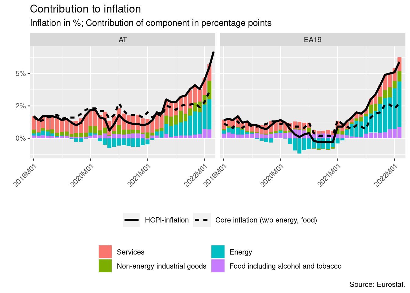
This post was inspired by a graph used in OeNB (June 2020). Gesamtwirtschaftliche Prognose der OeNB für Österreich 2020 bis 2023. https://www.oenb.at/dam/jcr:613c5956-9909-455a-8d57-2cd480179774/prognose_juni_2020.pdf