Stochastic Frontier Models in R
with tags stochastic-frontier efficiency production-function maximum-likelihood panel-dataAn OLS regression describes the average relationship between inputs and output. But in many economic questions the average is not what we are interested in. If two firms use the same amount of capital and labour, but one produces twice as much as the other, we would like to know how far each of them is away from what is technically possible – and not from what is usual. Stochastic frontier models, which were proposed independently by Aigner, Lovell and Schmidt (1977) and Meeusen and van den Broeck (1977), are designed for exactly that question. This post introduces the basic idea behind them and shows how to estimate such models in R.
The idea behind a frontier
Consider the following artificial sample of 300 firms, which use a single input to produce a single output. Both variables are measured in logarithms.
# Reset random number generator for reproducibility
set.seed(1234)

# Number of firms
N <- 300

# Log input
lx <- log(runif(N, 5, 100))

# Symmetric noise, e.g. weather, measurement error or luck
v <- rnorm(N, 0, .15)

# One-sided inefficiency term, which can only be positive
u <- abs(rnorm(N, 0, .35))

# Log output
ly <- 1 + .6 * lx + v - u

sim <- data.frame(ly = ly, lx = lx)
The sample was generated from the relationship \(ly_i = 1 + 0.6 lx_i + v_i - u_i\), where \(v_i\) is a standard error term, which can be positive or negative, and \(u_i\) is a term that is never negative. The latter pushes every firm below the line, which describes the maximum attainable output. The following graph shows the sample together with the true frontier and the OLS regression line.
library(ggplot2)

ggplot(sim, aes(x = lx, y = ly)) +
  geom_point() +
  geom_abline(intercept = 1, slope = .6) +
  geom_smooth(method = "lm", se = FALSE, linetype = "dashed") +
  labs(x = "Log input", y = "Log output",
       title = "Frontier (solid) and OLS (dashed)") +
  theme_bw()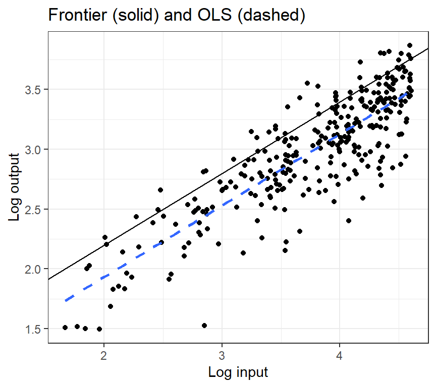
The two lines are practically parallel, but the OLS line lies clearly below the frontier. This is the central point: OLS goes through the point cloud, while the frontier is an upper envelope over it. Since the inefficiency term has a positive mean, OLS does not estimate the frontier, but the frontier minus average inefficiency. Its intercept is biased downwards, although the slope – and, hence, the elasticity of output with respect to the input – is still estimated consistently.
The model
The model behind the graph is \[y_i = \mathbf{x}_i^\prime \beta + v_i - u_i,\] where \(y_i\) is the log of output, \(\mathbf{x}_i\) contains the logs of the inputs, \(v_i \sim N(0, \sigma_v^2)\) is ordinary noise and \(u_i \geq 0\) measures technical inefficiency. The two error terms are assumed to be independent of each other and of the regressors. A common assumption for the one-sided term is the half-normal distribution, i.e. \(u_i \sim N^+(0, \sigma_u^2)\), which means that most firms are close to the frontier and only few are far below it.
Since \(u_i\) and \(v_i\) cannot be observed separately, the model is estimated by maximum likelihood, usually with the parameterisation of Battese and Coelli (1992) \[\sigma^2 = \sigma_v^2 + \sigma_u^2 \quad \text{and} \quad \gamma = \frac{\sigma_u^2}{\sigma_v^2 + \sigma_u^2},\] where \(\gamma\) lies between zero and one and indicates how important inefficiency is relative to noise.1 If \(\gamma\) is close to zero, the deviations from the frontier are pure noise and there is no reason to estimate anything else than OLS.
Once the model is estimated, the inefficiency of an individual firm can be predicted from its residual. The usual measure of technical efficiency is \[TE_i = \exp(-u_i),\] which is estimated by \(E[\exp(-u_i) | v_i - u_i]\) as proposed by Jondrow et al. (1982) and Battese and Coelli (1988). It takes values between zero and one, where one means that the firm produces on the frontier. A value of 0.8, for example, says that the firm produces 80 percent of the output that it could produce with its inputs.
Estimation in R
The frontier package of Arne Henningsen provides the function sfa, which is an R implementation of Tim Coelli’s FRONTIER 4.1 program. Applied to the artificial sample from above it gives
library(frontier) # install.packages("frontier")

sim_sfa <- sfa(ly ~ lx, data = sim)

summary(sim_sfa)
## Error Components Frontier (see Battese & Coelli 1992)
## Inefficiency decreases the endogenous variable (as in a production function)
## The dependent variable is logged
## Iterative ML estimation terminated after 6 iterations:
## log likelihood values and parameters of two successive iterations
## are within the tolerance limit
##
## final maximum likelihood estimates
## Estimate Std. Error z value Pr(>|z|)
## (Intercept) 1.007969 0.081451 12.3752 < 2.2e-16 ***
## lx 0.596251 0.020081 29.6930 < 2.2e-16 ***
## sigmaSq 0.134925 0.018208 7.4103 1.261e-13 ***
## gamma 0.829647 0.058451 14.1938 < 2.2e-16 ***
## ---
## Signif. codes: 0 '***' 0.001 '**' 0.01 '*' 0.05 '.' 0.1 ' ' 1
## log likelihood value: -5.847546
##
## cross-sectional data
## total number of observations = 300
##
## mean efficiency: 0.7809427The estimate of the intercept is much closer to its true value of one than the OLS estimate, which is
coef(lm(ly ~ lx, data = sim))## (Intercept) lx
## 0.7340934 0.5982447The difference between the two intercepts corresponds to the mean of the inefficiency term. For a half-normal distribution it is \(E[u_i] = \sigma_u \sqrt{2 / \pi}\) and, thus, about 0.28 in this sample. Note that separating two error terms, which are never observed individually, asks a lot of the data. In small samples the estimates of \(\gamma\) and of the intercept can be quite imprecise, and it can even happen that the estimation collapses to the OLS solution.
Example: production of 60 firms
The frontier package contains the cross section data set, which comes with FRONTIER 4.1. It consists of 60 firms and contains an index of output as well as indices of capital and labour input.
data("front41Data")

head(front41Data)
## firm output capital labour
## 1 1 12.778 9.416 35.134
## 2 2 24.285 4.643 77.297
## 3 3 20.855 5.095 89.799
## 4 4 13.213 4.935 35.698
## 5 5 12.018 8.717 27.878
## 6 6 15.284 1.066 92.174Since all variables enter the model in logarithms, the following specification is a Cobb-Douglas production frontier, where the coefficients can be interpreted as output elasticities and their sum measures the returns to scale.
cobb_douglas <- sfa(log(output) ~ log(capital) + log(labour),
                    data = front41Data)

summary(cobb_douglas)
## Error Components Frontier (see Battese & Coelli 1992)
## Inefficiency decreases the endogenous variable (as in a production function)
## The dependent variable is logged
## Iterative ML estimation terminated after 7 iterations:
## log likelihood values and parameters of two successive iterations
## are within the tolerance limit
##
## final maximum likelihood estimates
## Estimate Std. Error z value Pr(>|z|)
## (Intercept) 0.561619 0.202617 2.7718 0.0055742 **
## log(capital) 0.281102 0.047643 5.9001 3.632e-09 ***
## log(labour) 0.536480 0.045252 11.8555 < 2.2e-16 ***
## sigmaSq 0.217000 0.063909 3.3955 0.0006851 ***
## gamma 0.797207 0.136424 5.8436 5.109e-09 ***
## ---
## Signif. codes: 0 '***' 0.001 '**' 0.01 '*' 0.05 '.' 0.1 ' ' 1
## log likelihood value: -17.02722
##
## cross-sectional data
## total number of observations = 60
##
## mean efficiency: 0.7405678Is there inefficiency at all?
Before the efficiency estimates are interpreted, it should be checked whether the data actually support a frontier model. The null hypothesis \(\gamma = 0\) means that there is no inefficiency and that OLS would be the appropriate estimator. The lrtest function compares the estimated frontier with the corresponding OLS model:
lrtest(cobb_douglas)## Likelihood ratio test
##
## Model 1: OLS (no inefficiency)
## Model 2: Error Components Frontier (ECF)
## #Df LogLik Df Chisq Pr(>Chisq)
## 1 4 -18.447
## 2 5 -17.027 1 2.8392 0.04599 *
## ---
## Signif. codes: 0 '***' 0.001 '**' 0.01 '*' 0.05 '.' 0.1 ' ' 1Note that under the null hypothesis the parameter \(\gamma\) lies on the boundary of the parameter space. Therefore, the test statistic does not follow a standard \(\chi^2\) distribution, but a mixed \(\chi^2\) distribution, which the function takes into account. A rejection of the null hypothesis means that the deviations from the frontier are systematic and not only noise. In this example the null hypothesis is rejected at the 5 percent level, but not by a wide margin. This is not unusual for a sample of 60 observations.
Technical efficiency scores
The efficiency of each firm is obtained with the efficiencies function:
eff <- efficiencies(cobb_douglas)

summary(as.numeric(eff))
## Min. 1st Qu. Median Mean 3rd Qu. Max.
## 0.3513 0.6772 0.7585 0.7406 0.8428 0.9374ggplot(data.frame(eff = as.numeric(eff)), aes(x = eff)) +
geom_histogram(bins = 15) +
labs(x = "Technical efficiency", y = "Number of firms") +
theme_bw()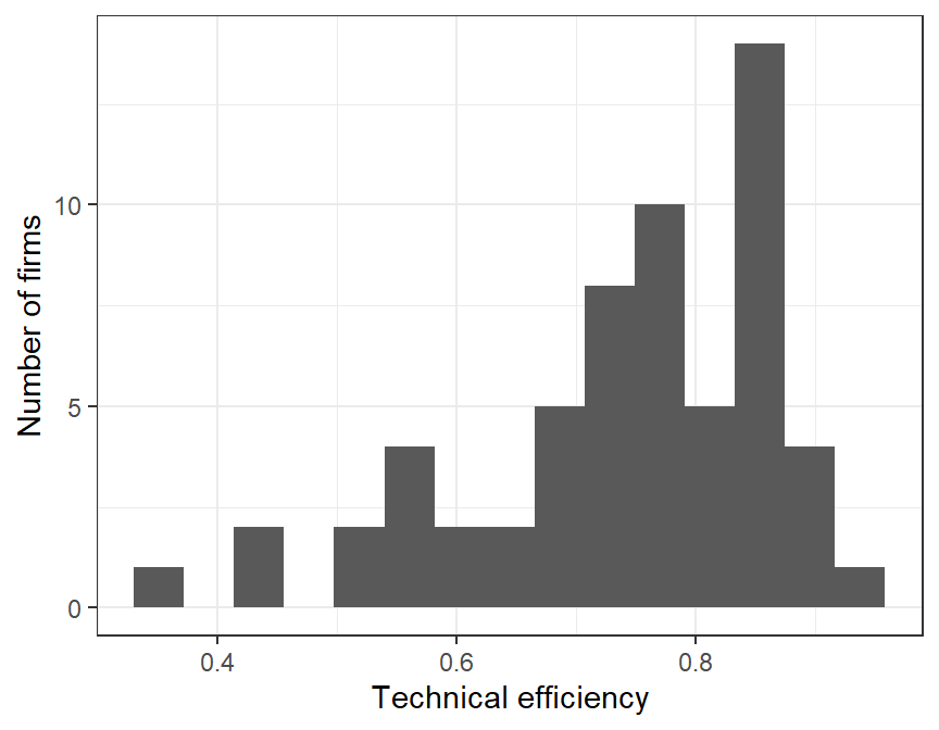
The distribution of these estimates is what makes the approach attractive for applied work. It does not only say how efficient the average firm is, but also which firms could increase their output most without using more inputs. However, the individual estimates are predictions of an unobserved random variable and, therefore, relatively imprecise. They should be interpreted with care, especially when they are used to rank firms.
Where does inefficiency come from?
For most applications the more interesting question is not how much inefficiency there is, but why. Battese and Coelli (1995) proposed a model, in which the mean of the inefficiency term depends on a set of explanatory variables \(\mathbf{z}_i\), i.e. \[u_i \sim N^+(\mathbf{z}_i^\prime \delta, \sigma_u^2).\] The frontier and the inefficiency effects are estimated in a single step. This avoids the inconsistencies of the older two-step approach, where the estimated efficiencies are regressed on \(\mathbf{z}\) in a second regression.
The frontier package also contains a data set of 43 smallholder rice producers in the Philippines, which were observed between 1990 and 1997. It is the example, which is used in Coelli et al. (2005). Panel data have to be prepared with the pdata.frame function of the plm package, where the first variable identifies the farmer and the second the time period.
library(plm) # install.packages("plm")

data("riceProdPhil")

rice_panel <- pdata.frame(riceProdPhil, c("FMERCODE", "YEARDUM"))
The variables of the production frontier are output PROD in tonnes, land AREA in hectares, LABOR in man-days and fertiliser NPK in kilogram. The inefficiency effects are separated from the frontier by a vertical bar |. In this example the years of education of the household head EDYRS and the share of upland fields BANRAT are assumed to affect inefficiency.
rice <- sfa(log(PROD) ~ log(AREA) + log(LABOR) + log(NPK) | EDYRS + BANRAT,
            data = rice_panel)

summary(rice)
## Efficiency Effects Frontier (see Battese & Coelli 1995)
## Inefficiency decreases the endogenous variable (as in a production function)
## The dependent variable is logged
## Iterative ML estimation terminated after 47 iterations:
## log likelihood values and parameters of two successive iterations
## are within the tolerance limit
##
## final maximum likelihood estimates
## Estimate Std. Error z value Pr(>|z|)
## (Intercept) -1.051760 0.252990 -4.1573 3.220e-05 ***
## log(AREA) 0.379767 0.059976 6.3319 2.421e-10 ***
## log(LABOR) 0.321029 0.061125 5.2520 1.505e-07 ***
## log(NPK) 0.263797 0.034458 7.6555 1.926e-14 ***
## Z_(Intercept) -2.746459 8.499206 -0.3231 0.7466
## Z_EDYRS -0.028610 0.215997 -0.1325 0.8946
## Z_BANRAT -3.635528 8.096598 -0.4490 0.6534
## sigmaSq 1.666588 3.695879 0.4509 0.6520
## gamma 0.978799 0.045203 21.6536 < 2.2e-16 ***
## ---
## Signif. codes: 0 '***' 0.001 '**' 0.01 '*' 0.05 '.' 0.1 ' ' 1
## log likelihood value: -77.31363
##
## panel data
## number of cross-sections = 43
## number of time periods = 8
## total number of observations = 344
## thus there are 0 observations not in the panel
##
## mean efficiency of each year
## 1 2 3 4 5 6 7 8
## 0.7619359 0.7505762 0.8311524 0.8118776 0.7641510 0.8081221 0.7049660 0.8466347
##
## mean efficiency: 0.784927The coefficients of the z variables require some attention, because they describe the effect on inefficiency and not on efficiency. A negative coefficient means that the variable reduces inefficiency and, therefore, increases output. Both estimates are negative, which would suggest that better educated farmers and farmers with a larger share of upland fields operate closer to the frontier. However, neither of them is significantly different from zero. With 43 farmers and explanatory variables, which hardly change over time, this is a fairly common outcome. It is a useful reminder that the inefficiency effects model identifies the \(\delta\) parameters from the asymmetry of the residuals, which is a much weaker source of information than the variation that identifies the coefficients of the frontier itself.
Since the model allows the mean of the inefficiency term to differ across observations, the efficiency estimates also vary over time. The output above reports the mean efficiency for each of the eight years. The individual estimates can be added to the data in the order of the observations, which is convenient for further analysis:
rice_panel$efficiency <- efficiencies(rice, asInData = TRUE)

summary(as.numeric(rice_panel$efficiency))
## Min. 1st Qu. Median Mean 3rd Qu. Max.
## 0.1399 0.7255 0.8311 0.7849 0.8874 0.9585Cost frontiers
So far, inefficiency reduced output. In a cost function it works the other way round, because an inefficient firm has higher costs than necessary. This only requires to set the argument ineffDecrease = FALSE, which flips the sign of the one-sided error term.
rice_panel$cost <- rice_panel$LABOR * rice_panel$LABORP +
  rice_panel$NPK * rice_panel$NPKP

rice_cost <- sfa(log(cost) ~ log(PROD) + log(AREA) + log(LABORP) + log(NPKP),
                 data = rice_panel, ineffDecrease = FALSE)

summary(rice_cost)
## Error Components Frontier (see Battese & Coelli 1992)
## Inefficiency increases the endogenous variable (as in a cost function)
## The dependent variable is logged
## Iterative ML estimation terminated after 13 iterations:
## log likelihood values and parameters of two successive iterations
## are within the tolerance limit
##
## final maximum likelihood estimates
## Estimate Std. Error z value Pr(>|z|)
## (Intercept) 5.802370 0.187152 31.0034 < 2.2e-16 ***
## log(PROD) 0.371840 0.034212 10.8688 < 2.2e-16 ***
## log(AREA) 0.553136 0.037770 14.6447 < 2.2e-16 ***
## log(LABORP) 0.443487 0.031269 14.1829 < 2.2e-16 ***
## log(NPKP) 0.091793 0.053321 1.7215 0.0851602 .
## sigmaSq 0.072843 0.015707 4.6376 3.524e-06 ***
## gamma 0.482776 0.125711 3.8404 0.0001229 ***
## ---
## Signif. codes: 0 '***' 0.001 '**' 0.01 '*' 0.05 '.' 0.1 ' ' 1
## log likelihood value: 49.36599
##
## panel data
## number of cross-sections = 43
## number of time periods = 8
## total number of observations = 344
## thus there are 0 observations not in the panel
##
## mean efficiency: 0.8593954Further options
The half-normal distribution of the inefficiency term is a convenient assumption, but not the only one. The argument truncNorm = TRUE allows for a truncated normal distribution, which adds a parameter \(\mu\) and makes the model more flexible, and timeEffect = TRUE allows efficiency to change over time in panel models. If more distributions are required, the sfaR package provides ten of them – among others the exponential, gamma, lognormal and Weibull distribution – as well as latent class and sample selection models. A non-parametric alternative to the whole approach is data envelopment analysis (DEA), which is implemented in the Benchmarking package. It does not require a functional form, but it also does not distinguish between inefficiency and noise.
Literature
Aigner, D., Lovell, C. A. K., & Schmidt, P. (1977). Formulation and estimation of stochastic frontier production function models. Journal of Econometrics, 6(1), 21–37.
Battese, G. E., & Coelli, T. J. (1988). Prediction of firm-level technical efficiencies with a generalized frontier production function and panel data. Journal of Econometrics, 38(3), 387–399.
Battese, G. E., & Coelli, T. J. (1992). Frontier production functions, technical efficiency and panel data: With application to paddy farmers in India. Journal of Productivity Analysis, 3(1), 153–169.
Battese, G. E., & Coelli, T. J. (1995). A model for technical inefficiency effects in a stochastic frontier production function for panel data. Empirical Economics, 20(2), 325–332.
Coelli, T. J. (1996). A guide to FRONTIER version 4.1: A computer program for stochastic frontier production and cost function estimation. CEPA Working Paper 96/08, University of New England.
Coelli, T. J., Rao, D. S. P., O’Donnell, C. J., & Battese, G. E. (2005). An introduction to efficiency and productivity analysis (2nd ed.). New York: Springer.
Henningsen, A. (2020). frontier: Stochastic frontier analysis. R package version 1.1-8.
Jondrow, J., Lovell, C. A. K., Materov, I. S., & Schmidt, P. (1982). On the estimation of technical inefficiency in the stochastic frontier production function model. Journal of Econometrics, 19(2–3), 233–238.
Kumbhakar, S. C., & Lovell, C. A. K. (2000). Stochastic frontier analysis. Cambridge: Cambridge University Press.
Meeusen, W., & van den Broeck, J. (1977). Efficiency estimation from Cobb-Douglas production functions with composed error. International Economic Review, 18(2), 435–444.
Strictly speaking, \(\gamma\) is not the share of the total error variance, which is due to inefficiency, because the variance of a half-normal variable is \((1 - 2 / \pi) \sigma_u^2\) and not \(\sigma_u^2\). It is a monotonic indicator, though. The closer it is to one, the more of the deviation from the frontier is systematic.↩︎
