Reproduction: Coelli, T. J. (1996). A guide to FRONTIER Version 4.1.
with tags r bsfa frontier stochastic-frontier efficiency production-function bayesian maximum-likelihoodFor most of the 1990s and 2000s, estimating a stochastic frontier meant running FRONTIER 4.1, Tim Coelli’s Fortran program, and its guide (Coelli, 1996) was where one learnt how. The guide works through a small example: a Cobb-Douglas production frontier for 60 firms with half-normal inefficiency, estimated by maximum likelihood. Its data are distributed with the program and, today, with the R package frontier by Coelli and Henningsen, which implements FRONTIER 4.1 in R.
This post reproduces that example twice: by maximum likelihood with frontier, which returns the guide’s printed estimates, and by Bayesian inference with bsfa. The second is the more interesting exercise, because the two approaches answer slightly different questions, and a sample of 60 is small enough for the difference to show.
The model
For firm \(i\) the frontier is
\[\ln Q_i = \beta_0 + \beta_1 \ln K_i + \beta_2 \ln L_i + v_i - u_i,\]
with output \(Q\), capital \(K\) and labour \(L\), a symmetric error \(v_i \sim N(0, \sigma_v^2)\) and a half-normal inefficiency term \(u_i \sim N^+(0, \sigma_u^2)\), so that the technical efficiency of firm \(i\) is \(\exp(-u_i)\). FRONTIER does not estimate \(\sigma_u^2\) and \(\sigma_v^2\) directly. It uses the parameterisation of Battese and Corra (1977),
\[\sigma^2 = \sigma_u^2 + \sigma_v^2, \qquad \gamma = \frac{\sigma_u^2}{\sigma^2},\]
in which \(\gamma\) lies between zero and one and measures how much of the composed error is inefficiency.
Maximum likelihood
library("frontier") # install.packages("frontier")
library("bsfa")     # remotes::install_github("franzmohr/bsfa")

data("front41Data", package = "frontier")
head(front41Data)
## firm output capital labour
## 1 1 12.778 9.416 35.134
## 2 2 24.285 4.643 77.297
## 3 3 20.855 5.095 89.799
## 4 4 13.213 4.935 35.698
## 5 5 12.018 8.717 27.878
## 6 6 15.284 1.066 92.174ml <- sfa(log(output) ~ log(capital) + log(labour), data = front41Data)
summary(ml)## Error Components Frontier (see Battese & Coelli 1992)
## Inefficiency decreases the endogenous variable (as in a production function)
## The dependent variable is logged
## Iterative ML estimation terminated after 7 iterations:
## log likelihood values and parameters of two successive iterations
## are within the tolerance limit
##
## final maximum likelihood estimates
## Estimate Std. Error z value Pr(>|z|)
## (Intercept) 0.561619 0.202617 2.7718 0.0055742 **
## log(capital) 0.281102 0.047643 5.9001 3.632e-09 ***
## log(labour) 0.536480 0.045252 11.8555 < 2.2e-16 ***
## sigmaSq 0.217000 0.063909 3.3955 0.0006851 ***
## gamma 0.797207 0.136424 5.8436 5.109e-09 ***
## ---
## Signif. codes: 0 '***' 0.001 '**' 0.01 '*' 0.05 '.' 0.1 ' ' 1
## log likelihood value: -17.02722
##
## cross-sectional data
## total number of observations = 60
##
## mean efficiency: 0.7405678These are the guide’s estimates: \(\hat\beta_0 = 0.5616\), \(\hat\beta_1 = 0.2811\), \(\hat\beta_2 = 0.5365\), \(\hat\sigma^2 = 0.2170\) and \(\hat\gamma = 0.7972\), with a log-likelihood of \(-17.027\) and a mean technical efficiency of
mean(efficiencies(ml))## [1] 0.7405678Bayesian inference
bsfa samples the same model by data augmentation: the inefficiency terms are drawn as latent variables, and the frontier and the variances are drawn given them. The coefficients get a flat prior, so that they are left to the data. The inefficiency term cannot be treated that way: its prior is elicited from a prior median efficiency, 0.75 by default, in the manner of van den Broeck, Koop, Osiewalski and Steel (1994).
model <- create_sfmodel_hn(log(output) ~ log(capital) + log(labour),
                           data = front41Data,
                           iterations = 20000,
                           burnin = 5000)

model <- add_priors(model, coef = list(mu = 0, v_i = 1e-6))

model <- add_posterior_coefficients(add_seed(model, 1996))

summary(model)
## Bayesian stochastic frontier model
##
## Call:
## create_sfmodel_hn(formula = log(output) ~ log(capital) + log(labour),
## data = front41Data, iterations = 20000, burnin = 5000)
##
## Frontier: production
## Inefficiency: halfnormal
## Observations: 60
## Units: 60
## Draws: 20000 after 5000 burn-in, thinning 1
##
## Posterior summary, 95% credible bands:
## mean sd 2.5% median 97.5% ESS
## (Intercept) 0.5679 0.2136 0.1531 0.5655 0.9965 4023
## log(capital) 0.2801 0.0498 0.1804 0.2810 0.3747 5056
## log(labour) 0.5331 0.0484 0.4363 0.5338 0.6267 6305
## sigma_v 0.2326 0.0482 0.1477 0.2295 0.3348 1332
## sigma_u 0.4080 0.0788 0.2617 0.4046 0.5718 1013
## sigma_u/sigma_v 1.8759 0.6858 0.8540 1.7668 3.4993 989
##
## Posterior mean efficiency, per observation:
## mean min median max
## 0.7464 0.3923 0.7603 0.9298The frontier coefficients agree with the maximum likelihood estimates to within a small fraction of a standard error, and their posterior standard deviations are close to the guide’s standard errors of 0.203, 0.048 and 0.045. That is what a flat prior on the coefficients should deliver.
The variance parameters are a different matter. Translated into FRONTIER’s parameterisation, draw by draw:
su2 <- as.numeric(model[["posterior"]][["sigma_u"]][["coeffs"]])^2
sv2 <- as.numeric(model[["posterior"]][["sigma_v"]][["coeffs"]])^2

sigma_sq <- su2 + sv2
gamma_ratio <- su2 / sigma_sq

rbind(sigma_sq = quantile(sigma_sq, c(0.025, 0.5, 0.975)),
      gamma = quantile(gamma_ratio, c(0.025, 0.5, 0.975)))
## 2.5% 50% 97.5%
## sigma_sq 0.1422667 0.2197297 0.3683003
## gamma 0.4217152 0.7573677 0.9245013\(\sigma^2\) is estimated much as by maximum likelihood, but \(\gamma\) is not pinned down: its 95 per cent credible interval runs over half the unit interval. The maximum likelihood standard error of 0.136 says the same, if less plainly, and it is the honest answer for a sample of 60. How the composed error splits into noise and inefficiency is identified only through the asymmetry of the residuals, and 60 residuals do not carry much of it. The posterior median lies a little below \(\hat\gamma\) because the posterior is skewed towards the lower values, and a mode and a median of a skewed distribution are not the same point.
Efficiency
The mean efficiency agrees closely:
eff <- efficiency(model)
mean(eff[["mean"]])
## [1] 0.7463599What the Bayesian fit adds is the uncertainty around each firm’s score. The maximum likelihood estimates of efficiency are the conditional expectations of Battese and Coelli (1988), evaluated at the point estimates; the posterior means above are the same expectation, averaged over the uncertainty in the parameters as well, and each comes with a credible interval.
plot(model, type = "efficiency", units = 60)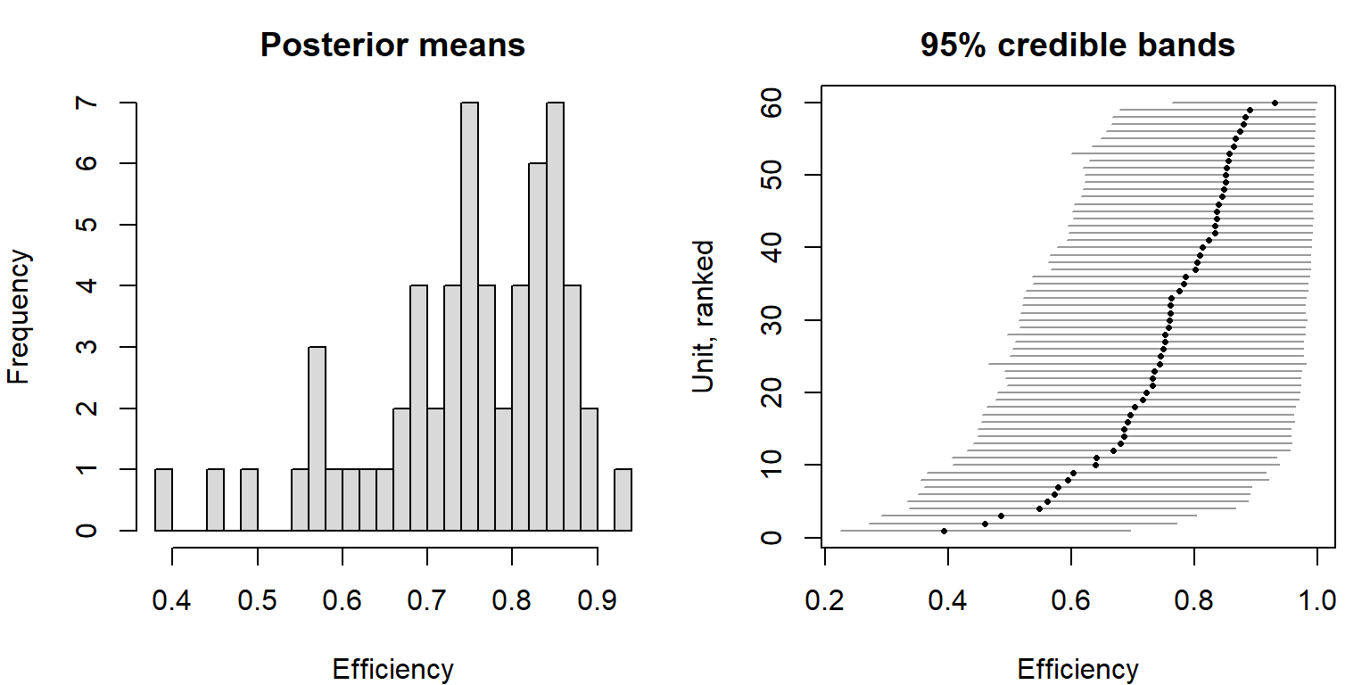
Most intervals are wide. With one observation per firm there is little information about any single firm’s inefficiency, and a ranking of the 60 firms by their point scores would suggest far more precision than the data contain.
References
Battese, G. E., & Coelli, T. J. (1988). Prediction of firm-level technical efficiencies with a generalized frontier production function and panel data. Journal of Econometrics, 38(3), 387–399.
Battese, G. E., & Corra, G. S. (1977). Estimation of a production frontier model: With application to the pastoral zone of Eastern Australia. Australian Journal of Agricultural Economics, 21(3), 169–179.
Coelli, T. J. (1996). A guide to FRONTIER Version 4.1: A computer program for stochastic frontier production and cost function estimation. CEPA Working Paper 96/07. Armidale: University of New England.
Coelli, T., & Henningsen, A. (2020). frontier: Stochastic frontier analysis. R package. https://CRAN.R-project.org/package=frontier
van den Broeck, J., Koop, G., Osiewalski, J., & Steel, M. F. J. (1994). Stochastic frontier models: A Bayesian perspective. Journal of Econometrics, 61(2), 273–303. https://doi.org/10.1016/0304-4076(94)90087-6
