Reproduction: Koop, G., León-González, R., & Strachan, R. W. (2011). Bayesian inference in a time varying cointegration model.

The model

For an \(n \times 1\) vector \(y_t\) the measurement equation is

\[\Delta y_t = \alpha_t \beta_t^{\prime} y_{t-1} + \sum_{h=1}^{l} \Gamma_{h,t} \Delta y_{t-h} + \Phi_t d_t + \varepsilon_t, \quad \varepsilon_t \sim N(0, \Omega_t),\]

where \(\alpha_t\) and \(\beta_t\) are \(n \times r\) and \(\beta_t\) is semi-orthogonal, \(\beta_t^{\prime} \beta_t = I_r\), so that it identifies the space \(\mathfrak{p}_t = sp(\beta_t)\) without restricting it. Write \(\beta_t^* = \beta_t \kappa_t\) for an unrestricted matrix of cointegrating vectors, with \(\kappa_t = (\beta_t^{*\prime} \beta_t^*)^{1/2}\), and \(b_t^* = vec(\beta_t^*)\). The state equation of the cointegration space is

\[b_t^* = \rho b_{t-1}^* + \eta_t, \quad \eta_t \sim N(0, I_{nr}), \quad b_1^* \sim N\left(0, I_{nr} \frac{1}{1 - \rho^2}\right),\]

with \(|\rho| < 1\). The paper proves that under this equation the density of \(\mathfrak{p}_t\) given \(\mathfrak{p}_{t-1}\) has its mode, and in Villani’s (2006) sense its mean, at \(\mathfrak{p}_{t-1}\), and that \(\rho\) controls how concentrated it is around that location. A \(\rho\) close to one means small changes from one period to the next, and the paper’s prior restricts it to \([0.999, 1)\).

The remaining coefficients \(A_t = (\alpha_t^*, \Gamma_{1,t}, \ldots, \Gamma_{l,t}, \Phi_t)\), with \(\alpha_t^* = \alpha_t \kappa_t^{-1}\) so that \(\alpha_t^* \beta_t^{*\prime} = \alpha_t \beta_t^{\prime}\), follow a random walk, and \(\Omega_t\) is the stochastic volatility specification of Primiceri (2005): \(\Lambda_t \Omega_t \Lambda_t^{\prime} = \Sigma_t \Sigma_t^{\prime}\) with \(\Lambda_t\) unit lower triangular and \(\Sigma_t\) diagonal, and random walks for the free elements of \(\Lambda_t\) and the log standard deviations in \(\Sigma_t\).

The application is bivariate, \(y_t = (r_t, \pi_t)^{\prime}\), with one lag of differences and an intercept. Its models differ in which of the three blocks moves: \((d_\Omega, d_\beta, d_a)\) is one for a block that is time varying and zero for one that is constant, and the rank \(r\) is zero, one or two. Under the Fisher hypothesis \(r = 1\), and normalising the cointegrating vector as \((1, B_t)^{\prime}\) gives \(B_t = -1\).

The data

The paper uses quarterly UK data from the IMF’s International Financial Statistics: the Treasury bill rate and CPI inflation, annualised by multiplying the quarterly log difference by 400. They are included in bvartools as columns rs and Dp of data set uk_macrodata.

library("bvartools")
library("knitr")

data("uk_macrodata")
uk <- uk_macrodata[, c("rs", "Dp")]
colnames(uk) <- c("r", "pi")

plot(uk, main = "UK Treasury bill rate and inflation")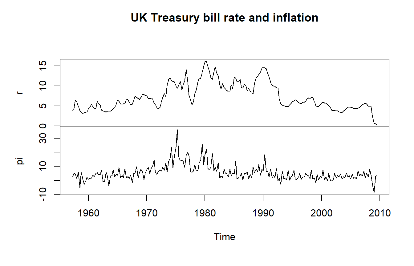

With one lag of differences the estimation sample runs from 1957 Q4 to 2009 Q3, 208 observations.

Priors

Appendix A of the paper gives the priors. bvartools puts independent priors on the diagonal of the covariance matrices of the state equations where the paper uses Wishart priors on their inverses, so each of them is translated into gamma priors with the same degrees of freedom and scale: a diagonal element of a \(W(\nu, S^{-1})\) matrix is gamma distributed with shape \(\nu / 2\) and rate \(S_{ii} / 2\).

Parameter	Paper	bvartools
\(\rho\)	\(U[0.999, 1)\)	coint = list(rho = 0.9995, rho_min = 0.999, rho_max = 1)
\(a_0\)	\(N(0, 2V)\), \(V = I\) except \(1 - \rho^2\) for \(\alpha^*\)	v_i = 1 / 2 in coef, loadings \(1 / (2 (1 - \rho^2))\)
\(Q^{-1}\)	\(W(\dim(a) + 2, 0.0001 I)\)	shape \((\dim(a) + 2) / 2\), rate \(0.0001 / 2\)
\(\lambda_0\), \(C^{-1}\)	\(N(0, 2)\), \(W(3, 0.0001)\)	precision \(1/2\), shape \(3/2\), rate \(0.0001 / 2\)
\(h_0\), \(W^{-1}\)	\(N(0, 2 I)\), \(W(n + 2, 0.0001 I)\)	v_i = 1 / 8, shape = 2 and rate = 4 \times 0.0001 / 2 in sigma

The last row needs a word. The paper’s \(h_t\) is the log of a standard deviation, while bvartools models the log of a variance, which is twice that. Its prior variance and the variance of its state equation are therefore four times as large.

A time varying cointegration space

A VEC model with tvp = TRUE lets every coefficient follow a random walk, and with error = "sv+covar" it is the model \((d_\Omega, d_\beta, d_a) = (1, 1, 1)\). add_priors takes most of the priors of the table directly, and the prior of the loadings and the shape of the prior of the covariance coefficient are set afterwards.

The paper’s preferred model, \((1, 1, 0)\), keeps \(A\) constant while the cointegration space moves. bvartools has no switch for that, but it does not need one: a gamma prior on the precision of the state equation of \(A\) with shape \(10^6\) and rate \(10^{-6}\) puts its variance at \(10^{-12}\), and the path of \(A\) is then constant to seven digits. That this gives a constant coefficient rather than a chain that stops moving depends on how the state before the sample is drawn. bvartools integrates it out of the prior of the first period, so the level of the path is left to the data.

One function sets up both models:

rho_0 <- 0.9995

tvp_vec <- function(series, d_omega, d_a, r = 1, iterations = 36000,
                    burnin = 1000) {

  sv <- d_omega == 1

  model <- create_bvecmodel(series,
                            p = 2,
                            r = r,
                            const = "unrestricted",
                            tvp = TRUE,
                            error = if (sv) "sv+covar" else "wishart",
                            iterations = iterations,
                            burnin = burnin)

  if (sv) {
    sigma <- list(mu = 0,
                  v_i = 1 / 8,
                  shape = 2,
                  rate = 4 * 0.0001 / 2,
                  state_variance = 0.001,
                  offset = 1e-8)
  } else {
    sigma <- list(df = "k + 1", scale = 1)
  }

  model <- add_priors(model,
                      coef = list(v_i = 1 / 2,
                                  v_i_det = 1 / 2,
                                  shape = 1,
                                  rate = 1),
                      coint = list(rho = rho_0, rho_min = 0.999, rho_max = 1),
                      sigma = sigma)

  # The loadings' prior precision, and the state equation of A
  k <- ncol(series)
  prior_a <- model[["priors"]][["a"]]
  n_a <- nrow(prior_a[["shape"]])

  diag(prior_a[["v_inv"]])[1:(k * r)] <- 1 / (2 * (1 - rho_0^2))

  if (d_a == 1) {
    prior_a[["shape"]][] <- (n_a + 2) / 2
    prior_a[["rate"]][] <- 0.0001 / 2
  } else {
    prior_a[["shape"]][] <- 1e6
    prior_a[["rate"]][] <- 1e-6
  }

  model[["priors"]][["a"]] <- prior_a

  if (sv) {
    model[["priors"]][["psi"]][["shape"]][] <- 3 / 2
    model[["priors"]][["psi"]][["rate"]][] <- 0.0001 / 2
  }

  return(model)
}

The paper runs its sampler for 1,000 burn-in draws and keeps the next 36,000. So does this post, which takes well under a minute per model.

set.seed(20110816)

model_110 <- tvp_vec(uk, d_omega = 1, d_a = 0)
model_110 <- add_initial_values(model_110)
model_110 <- add_posterior_coefficients(model_110)

set.seed(20110816)

model_111 <- tvp_vec(uk, d_omega = 1, d_a = 1)
model_111 <- add_initial_values(model_111)
model_111 <- add_posterior_coefficients(model_111)

The cointegrating coefficient

The draws of \(b_t^*\) are in posterior[["beta"]][["coeffs"]], one pair of columns per period, and the normalised coefficient \(B_t = \beta_{2,t}^* / \beta_{1,t}^*\) is their ratio. It does not depend on the scale of \(b_t^*\), which is not identified.

b_ratio <- function(model, probs = c(0.05, 0.5, 0.95)) {

  beta_draws <- model[["posterior"]][["beta"]][["coeffs"]]
  odd <- seq(1, ncol(beta_draws), by = 2)
  b <- beta_draws[, odd + 1] / beta_draws[, odd]

  intervals <- t(apply(b, 2, quantile, probs = probs))

  return(ts(intervals,
            start = start(model[["data"]][["train"]][["y"]]),
            frequency = 4))
}

b_110 <- b_ratio(model_110)
b_111 <- b_ratio(model_111)

Fig. 1 of the paper plots the posterior median of \(B_t\) and its 90% credible interval for the preferred model:

ts.plot(b_110,
        lty = c(2, 1, 2),
        ylim = c(-7, 0),
        xlab = "",
        ylab = expression(B[t]),
        main = "Model (1, 1, 0), r = 1")

abline(h = -1)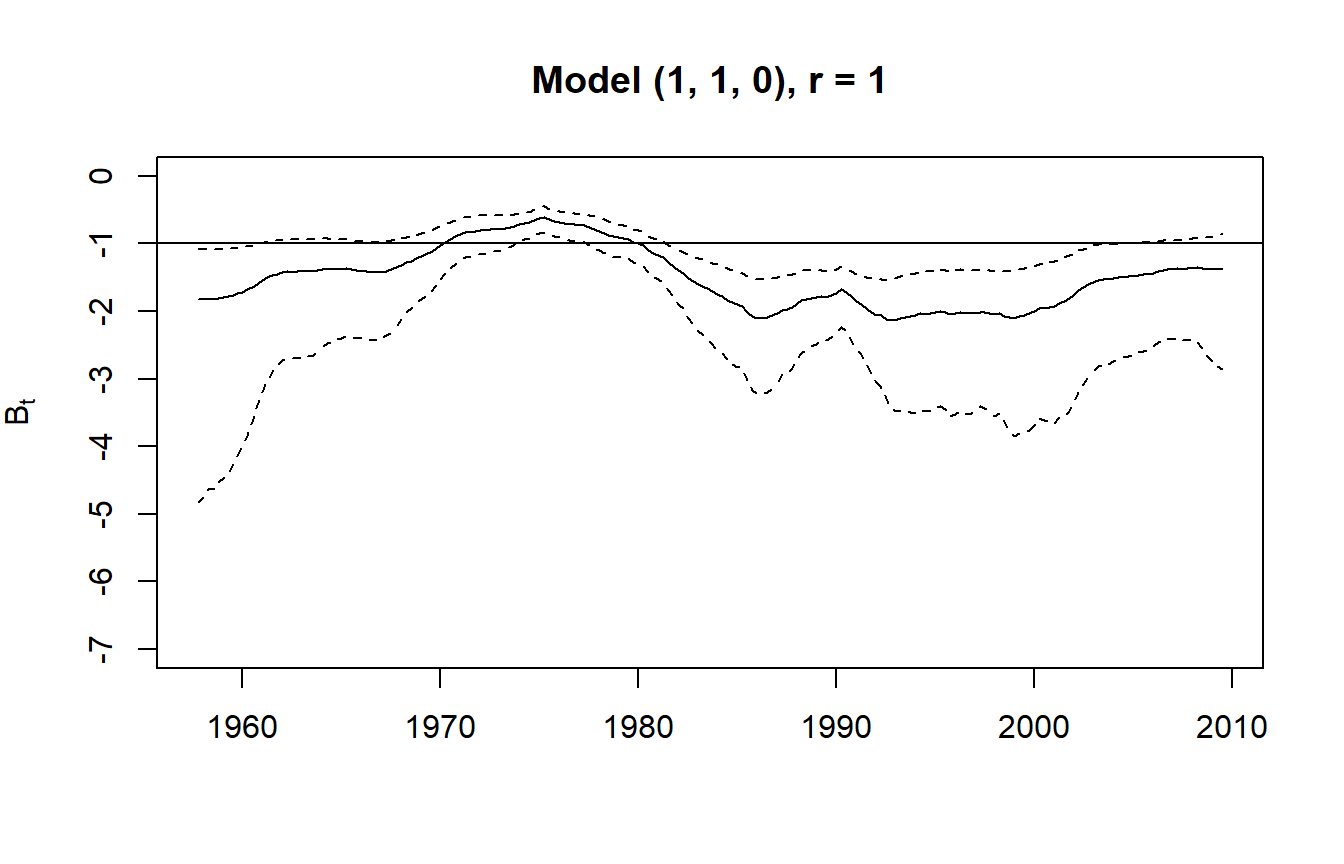

inside <- mean(b_110[, 1] <= -1 & b_110[, 3] >= -1)
below <- mean(b_110[, 3] < -1)

The path has the shape of the published one. The interval is wide at the start of the sample and lies below \(-1\), closes in on \(-1\) in the 1970s, drops to around \(-2\) in the 1980s and 1990s, and drifts back towards \(-1\) at the end of the sample. The paper reports that the interval contains \(-1\) in 34% of the periods and lies entirely below it in 60%. Here the shares are 43% and 50%: the interval is somewhat narrower and higher than in the paper, but the conclusion is the same. The Fisher hypothesis holds in some periods, most clearly in the 1970s, and not in others.

The model in which \(A\) drifts as well gives nearly the same path:

ts.plot(b_111,
        b_110,
        lty = c(2, 1, 2),
        col = rep(c("grey60", "black"), each = 3),
        ylim = c(-7, 0),
        xlab = "",
        ylab = expression(B[t]),
        main = "Models (1, 1, 1) and (1, 1, 0), r = 1")

abline(h = -1)

legend("bottomleft",
       legend = c("(1, 1, 1)", "(1, 1, 0)"),
       col = c("grey60", "black"),
       lty = 1,
       bty = "n")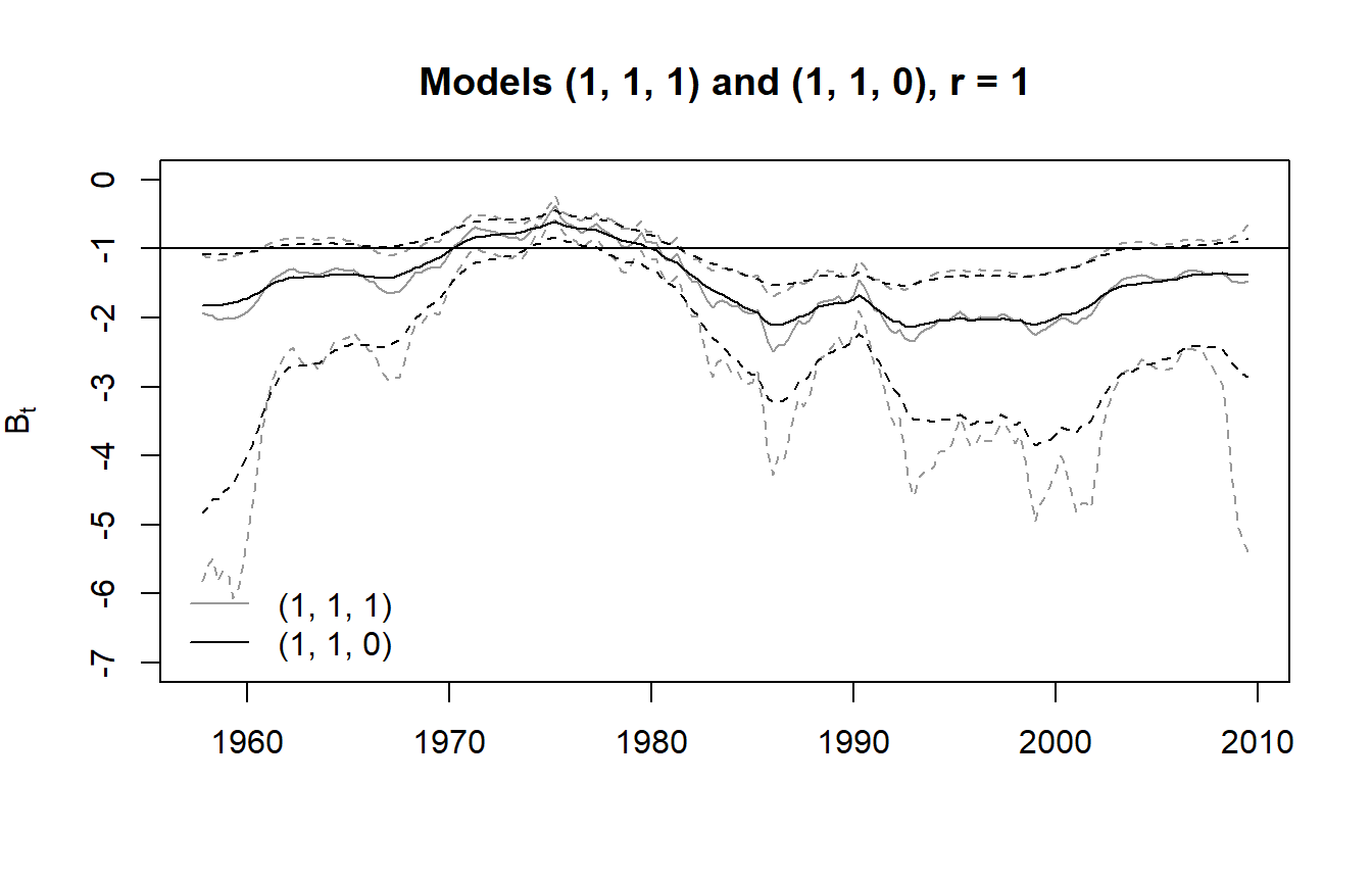

Predictive likelihoods

Tables 1 and 2 of the paper compare the models by the log predictive likelihood of the last 100 observations,

\[\sum_{t = T - 99}^{T} \ln p(\Delta y_t | y_{t-1}, \ldots, y_1).\]

Each term requires the model to be estimated on the data up to \(t - 1\). The states are then carried one period forward with their state equations, and the density of the realised \(\Delta y_t\) is averaged over 7,000 draws. That is 100 estimations per model and 1,600 in all, which is too slow to run while this page is built, so the code is shown and its results are loaded afterwards. For a VEC model estimated on the data up to \(t - 1\), one term is

last_period <- function(draws, size) {
  if (ncol(draws) == size) {
    return(draws)
  }
  return(draws[, ncol(draws) - size + 1:size, drop = FALSE])
}

# model: a VEC model estimated on the data up to t - 1
# obs:   the same model created on the data up to t, whose last rows hold
#        the realised Delta y_t and the regressors of period t
lpd_bvec <- function(model, obs, tvp_beta, tvp_a) {

  k <- model[["model"]][["k"]]
  r <- model[["model"]][["rank"]]

  train <- obs[["data"]][["train"]]
  n_obs <- nrow(train[["y"]])
  y <- as.numeric(train[["y"]][n_obs, ])
  w <- as.numeric(train[["w"]][n_obs, ])
  x <- as.numeric(train[["x"]][n_obs, ])

  post <- model[["posterior"]]

  # Carry the states one period forward
  a <- last_period(post[["a"]][["coeffs"]], k * (r + length(x)))
  if (tvp_a) {
    a <- a + matrix(rnorm(length(a)), nrow(a)) * sqrt(post[["a"]][["sigma"]])
  }

  beta_draws <- last_period(post[["beta"]][["coeffs"]], length(w) * r)
  if (tvp_beta) {
    beta_draws <- as.numeric(post[["beta"]][["rho"]]) * beta_draws +
      matrix(rnorm(length(beta_draws)), nrow(beta_draws))
  }

  prec <- last_period(post[["u_sigma_inv"]][["coeffs"]], k * k)

  # Log density of the realised Delta y_t, draw by draw
  ld <- sapply(seq_len(nrow(a)), function(i) {
    alpha <- matrix(a[i, 1:(k * r)], k)
    beta_i <- matrix(beta_draws[i, ], length(w))
    gamma_i <- matrix(a[i, -(1:(k * r))], k)
    mu <- alpha %*% crossprod(beta_i, w) + gamma_i %*% x

    p <- matrix(prec[i, ], k)
    log_det <- as.numeric(determinant(p)[["modulus"]])
    quad <- as.numeric(crossprod(y - mu, p %*% (y - mu)))

    return(-k / 2 * log(2 * pi) + 0.5 * log_det - 0.5 * quad)
  })

  return(max(ld) + log(mean(exp(ld - max(ld)))))
}

The models with a constant cointegration space are estimated with tvp = FALSE and a uniform prior on the space, coint = list(v_i = 0, p_tau_i = 1), and the models with \(r = 0\) as VARs in differences with create_bvarmodel.

The results of all models are in a small file next to this page:

lpl <- read.csv("_2011_kls_predlik.csv")
lpl[["label"]] <- paste0("r = ", lpl[["r"]], ", ", lpl[["model"]])

constant <- lpl[lpl[["label"]] %in% c("r = 1, (0,0,0)", "r = 0, (0,0)"), ]
constant[, c("label", "paper", "lpl100", "lpl110")]

##             label  paper lpl100 lpl110
## 8  r = 1, (0,0,0) -437.1 -392.9 -437.9
## 17   r = 0, (0,0) -442.5 -398.5 -442.5

Summed over the last 100 observations, the log predictive likelihoods of the two models with constant parameters are 44 higher than in the paper. Such models have nothing that could differ between two implementations beyond their priors, which 200 observations make irrelevant, and a gap that large means that the two sums are not over the same observations. Summed over the last 110, they agree with the published values to within 0.8. The paper’s sums therefore appear to run over 110 observations rather than the 100 its footnote states, and the comparison below uses 110.

format_lpl <- function(x, se) {
  return(ifelse(is.na(x), "not estimated", sprintf("%.1f (%.2f)", x, se)))
}

lpl_table <- data.frame(lpl[["r"]],
                        lpl[["model"]],
                        format_lpl(lpl[["paper"]], lpl[["paper_nse"]]),
                        format_lpl(lpl[["lpl110"]], lpl[["lpl110_nse"]]))

kable(lpl_table,
      col.names = c("$r$", "Model", "Paper", "bvartools"),
      align = "clrr")

\(r\)	Model	Paper	bvartools
1	(1,1,1)	-397.6 (0.66)	-400.1 (0.62)
1	(1,1,0)	-381.6 (0.61)	-383.6 (1.11)
1	(0,0,1)	-427.5 (0.14)	not estimated
1	(0,1,1)	-424.9 (0.12)	-425.7 (0.13)
1	(1,0,0)	-390.1 (0.86)	-396.0 (1.20)
1	(1,0,1)	-392.2 (0.72)	not estimated
1	(0,1,0)	-421.4 (0.08)	-420.6 (0.11)
1	(0,0,0)	-437.1 (0.05)	-437.9 (0.04)
2	(1,1,1)	-423.8 (0.93)	-418.9 (56.39)
2	(1,1,0)	-384.1 (0.58)	-385.9 (1.45)
2	(0,0,1)	-431.0 (0.97)	not estimated
2	(0,1,1)	-434.1 (1.10)	-423.2 (0.54)
2	(1,0,0)	-386.5 (1.11)	-395.8 (1.03)
2	(1,0,1)	-412.8 (1.21)	not estimated
2	(0,1,0)	-423.3 (0.12)	-421.9 (0.23)
2	(0,0,0)	-436.9 (0.05)	-437.6 (0.04)
0	(0,0)	-442.5 (0.04)	-442.5 (0.03)
0	(0,1)	-443.2 (0.05)	-442.7 (0.03)
0	(1,0)	-398.0 (0.62)	-407.9 (0.82)
0	(1,1)	-403.2 (0.59)	-408.4 (0.86)

The models are \((d_\Omega, d_\beta, d_a)\) for \(r > 0\) and \((d_\Omega, d_\Pi)\) for the VARs in differences, \(r = 0\). Numerical standard errors are in brackets.

est <- lpl[!is.na(lpl[["lpl110"]]), ]
best <- est[order(-est[["lpl110"]]), "label"]
rank_cor <- cor(est[["paper"]], est[["lpl110"]], method = "spearman")

The levels are not identical, which is to be expected with priors that are translated rather than copied and with a different sampler, but half of the estimated models are within 1.9 of the published value. What the paper’s conclusions rest on is the ordering, and it is reproduced: the rank correlation between the two columns is 0.99. The best model is r = 1, (1,1,0), followed by r = 2, (1,1,0) – the same two as in the paper – and the seven best models come in exactly the paper’s order. All seven have stochastic volatility, which is the feature that matters most. Among them, letting the short-run coefficients drift in addition to the cointegration space lowers the predictive likelihood in both ranks, and a constant cointegration space with stochastic volatility comes in between. The VARs in differences are dominated by the best cointegrated models.

The one estimate that should be read with care is that of r = 2, (1,1,1). Its numerical standard error is dominated by a single term, the one for 2008 Q4, when UK interest rates and inflation both fell sharply. An observation that far in the tail of the predictive density leaves its average to a handful of draws, and repeating that one term with different seeds moved it by as much as ten.

Deviations from the paper

• Priors on the state covariances. The paper uses Wishart priors on the inverse covariance matrices of the state equations of \(A_t\), \(\lambda_t\) and \(h_t\); they are replaced by independent gamma priors on the diagonal with the same degrees of freedom and scale.
• Constant coefficients. A block that is constant in the paper’s notation is a random walk with a state variance of \(10^{-12}\) here, not a constant parameter.
• \(\rho\). bvartools gives the state before the sample the stationary distribution at the starting value of \(\rho\), 0.9995, and keeps it there when \(\rho\) is drawn. That turns the draw of \(\rho\) into an exact Gibbs step, where the paper uses a Metropolis-within-Gibbs step.
• Constant error covariance. The paper does not state the prior of the models with a constant error covariance. Here it is inverse Wishart with \(n + 1\) degrees of freedom and an identity scale matrix.
• Predictive densities. The log volatilities and the covariance coefficient are held at their values in \(t - 1\) rather than carried forward with their state equations.
• Missing variants. The models \((1, 0, 1)\) and \((0, 0, 1)\) – drifting short-run coefficients with a constant cointegration space – are not estimated.

References

Koop, G., León-González, R., & Strachan, R. W. (2010). Efficient posterior simulation for cointegrated models with priors on the cointegration space. Econometric Reviews, 29(2), 224–242. https://doi.org/10.1080/07474930903382208

Koop, G., León-González, R., & Strachan, R. W. (2011). Bayesian inference in a time varying cointegration model. Journal of Econometrics, 165(2), 210–220. https://doi.org/10.1016/j.jeconom.2011.07.007

Primiceri, G. E. (2005). Time varying structural vector autoregressions and monetary policy. Review of Economic Studies, 72(3), 821–852. https://doi.org/10.1111/j.1467-937X.2005.00353.x

Villani, M. (2006). Bayesian point estimation of the cointegration space. Journal of Econometrics, 127(2), 645–664. https://doi.org/10.1016/j.jeconom.2005.01.002