Reproduction: Koop, G., & Korobilis, D. (2014). A new index of financial conditions.

The model

Let \(y_t\) be an \(n_y \times 1\) vector of macroeconomic variables and \(x_t\) an \(n_x \times 1\) vector of financial variables, from which a single unobserved factor \(f_t\) – the index – is extracted. The state vector is \(z_t = (y_t', f_t')'\) and the measurement equation is

\[\begin{bmatrix} y_t \\ x_t \end{bmatrix} = \begin{bmatrix} I & 0 \\ \lambda^y_t & \lambda^f_t \end{bmatrix} \begin{bmatrix} y_t \\ f_t \end{bmatrix} + \begin{bmatrix} 0 \\ e_t \end{bmatrix}, \quad e_t \sim N(0, V_t),\]

with \(V_t\) diagonal. The macroeconomic block is measured without error, which is why the corresponding block of the state is simply the data and only the factor has to be inferred. The financial variables load on the factor and on the macro variables, so \(\lambda^y_t\) removes from the index whatever is already explained by inflation, unemployment and output. That is the feature which distinguishes an FCI from a plain first principal component of financial data.

The transition equation is a VAR in the state,

\[z_t = \sum_{i=1}^{p} B_{i,t} z_{t-i} + u_t, \quad u_t \sim N(0, Q_t),\]

and both coefficient blocks follow random walks,

\[\lambda_t = \lambda_{t-1} + \epsilon_t, \quad \beta_t = \beta_{t-1} + \eta_t.\]

In a fully Bayesian treatment the variances of \(\epsilon_t\) and \(\eta_t\) would need priors of their own, and the model would have to be simulated. Koop and Korobilis (2014) instead follow Raftery et al. (2010) and pin the drift down with forgetting factors: the prediction variance of the coefficients in each block is inflated by a factor \(1 / \kappa\) at every step, so the amount of time variation is set by \(\kappa\) rather than estimated. The two error covariances \(V_t\) and \(Q_t\) are handled in the same spirit, as exponentially weighted moving averages of past squared residuals. Four tuning constants in total, and what is left is a filtering problem.

This is worth being explicit about, because it decides what may be read off the output. The Kalman recursions are exact Bayesian updating and the initial conditions are genuine priors, so the factor is a properly filtered quantity. Nothing to do with the variances is: the forgetting factors are plug-in point estimates substituted into the filter, and their uncertainty is discarded. fincond therefore returns one path per quantity, as ts objects rather than coda chains, and no interval computed from them is a credible interval. For a fully Bayesian dynamic factor model with priors on the innovation variances, bvartools is the appropriate tool instead.

The data

The package ships the paper’s data as koop.

library("fincond")

set.seed(1234567)

data("koop")

koop$financial holds the 18 financial series, quarterly from 1970 Q1 to 2013 Q3:

colnames(koop$financial)

##  [1] "sp500"          "twexmmth"       "oil"            "spread_ted"    
##  [5] "spread_10_2"    "spread_2_3m"    "spread_comm"    "loanhpi"       
##  [9] "spread_30_mort" "cmdebt"         "cci"            "move"          
## [13] "vix"            "totalsl"        "stdscom"        "mich1"         
## [17] "mich2"          "mich3"

Several of them start well after the sample does – the VIX in 1990, the MOVE index in 1988, the loan officer survey in 1990 – and are NA until they do:

colSums(is.na(koop$financial))

##          sp500       twexmmth            oil     spread_ted    spread_10_2 
##              0              0             17             47             26 
##    spread_2_3m    spread_comm        loanhpi spread_30_mort         cmdebt 
##             26              5             25              5              0 
##            cci           move            vix        totalsl        stdscom 
##              0             73             66              0             82 
##          mich1          mich2          mich3 
##              0              0              0

The macroeconomic block is a list of 96 real-time vintages of inflation (p), the unemployment rate (u) and output (y). Each vintage starts in 1970 Q1 and ends one quarter later than the one before it, so macro[[1]] ends in 1989 Q4 and macro[[96]] in 2013 Q3:

length(koop$macro)

## [1] 96

colnames(koop$macro[[96]])

## [1] "p" "u" "y"

rbind(first = end(koop$macro[[1]]), last = end(koop$macro[[96]]))

##       [,1] [,2]
## first 1989    4
## last  2013    3

The full sample index uses macro[[96]]. The earlier vintages are what the second exercise runs over.

The index

The model follows the workflow of bvartools: build the object, add priors, estimate.

model <- create_fcimodel(y = koop$macro[[96]], x = koop$financial,
                         p = 4, n = 1)
model <- add_priors(model)
model <- add_posterior_coefficients(model)

index <- fci(model, sign_on = "vix")

The sign and scale of a factor are not identified – multiplying the factor by \(-1\) and its loadings by \(-1\) leaves the model unchanged – so both have to be fixed by convention rather than estimated. sign_on = "vix" orients the index so that its loading on the VIX is positive, which makes a high value mean stressed conditions. That is a choice and not a result, and it has to be stated, because it decides whether a rising index means tightening or loosening.

plot(index, main = "Financial conditions index", ylab = "Index", xlab = "")
abline(h = 0, lty = "dashed", col = "grey40")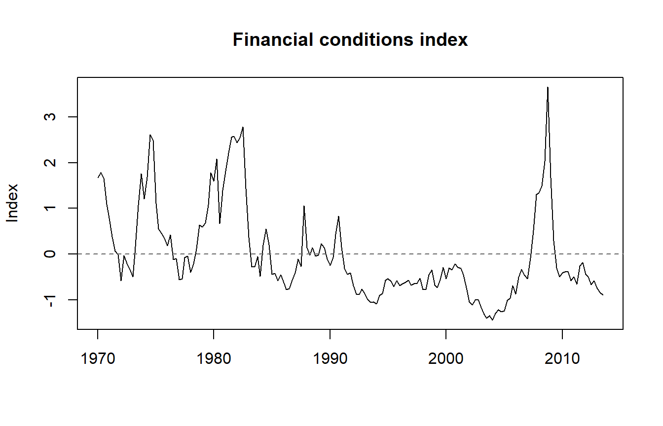

The paper’s headline claim concerns the ranking of episodes rather than any single value, so that is what to check it against. The eight highest readings:

as_quarter <- function(x) {
  yr <- floor(x)
  qtr <- round((x - yr) * 4) + 1
  paste0(yr, " Q", qtr)
}

ord <- order(-index)[1:8]

data.frame(quarter = as_quarter(as.numeric(time(index)))[ord],
           index = round(as.numeric(index)[ord], 2))

##   quarter index
## 1 2008 Q4  3.65
## 2 1982 Q3  2.78
## 3 1974 Q3  2.60
## 4 1981 Q4  2.57
## 5 1981 Q3  2.56
## 6 1982 Q2  2.54
## 7 1974 Q4  2.49
## 8 1982 Q1  2.44

The index peaks in 2008 Q4, ahead of the 1982 recession, the 1974 oil crisis and the 1981 tightening – the same ordering the paper reports. The three episodes that follow the 2008 peak are all clearly separated from it, which is the point: on this measure the financial crisis is not merely another bad quarter but the worst reading of the past four decades by a wide margin.

Factor loadings

Each financial series has its own time varying exposure to the index, and it is these paths that carry the paper’s argument about a changing financial system. plot(model, which = "loadings") draws them, one panel per series:

plot(model, which = "loadings")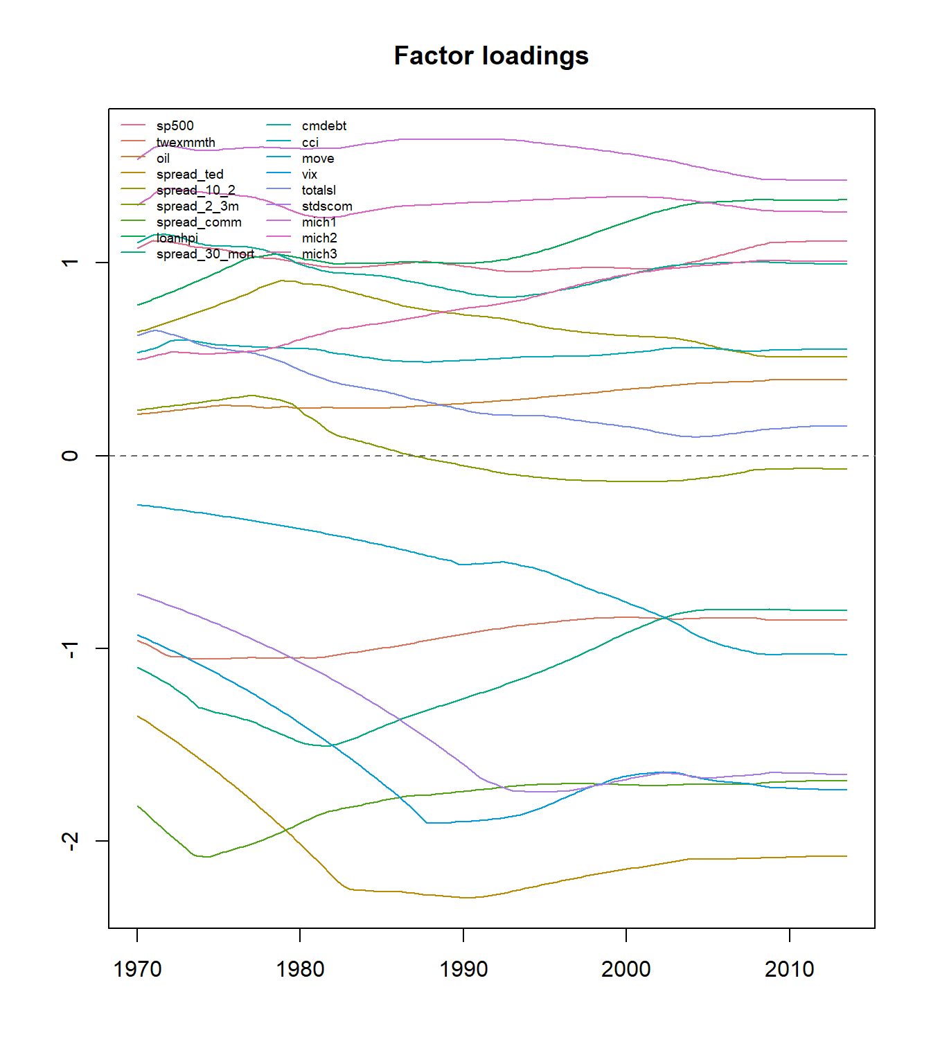

A loading drifting towards zero is a series the index has stopped drawing on. factor_loadings() returns the same paths as a matrix, so the first and last periods of the sample can be compared directly. Note that these are the loadings as estimated: the sign chosen in fci() is applied to the index it returns and is not written back into the model, so the whole matrix here carries the estimator’s own arbitrary orientation, which happens to be the mirror image of the VIX-oriented index plotted above. Read magnitudes, not signs.

loadings <- factor_loadings(model)

round(data.frame(first = loadings[1, ],
                 last = loadings[nrow(loadings), ]), 2)

##                first  last
## sp500           1.08  1.11
## twexmmth       -0.96 -0.85
## oil             0.21  0.39
## spread_ted     -1.35 -2.08
## spread_10_2     0.64  0.51
## spread_2_3m     0.24 -0.07
## spread_comm    -1.82 -1.69
## loanhpi         0.78  1.33
## spread_30_mort -1.10 -0.80
## cmdebt          1.10  0.99
## cci             0.53  0.55
## move           -0.25 -1.03
## vix            -0.93 -1.73
## totalsl         0.63  0.15
## stdscom        -0.72 -1.65
## mich1           1.54  1.43
## mich2           1.30  1.26
## mich3           0.50  1.01

The TED spread and the VIX both gain a lot of weight over the sample, and the MOVE index and the senior loan officer survey likewise – the four series that most directly measure funding stress and market volatility, and the ones a reader would expect a modern FCI to lean on. The stock market’s own contribution barely moves. That reweighting is the substantive result of allowing the loadings to drift: a constant-loading factor model would have had to average these two regimes into one.

A real-time index

Because the estimator needs no posterior simulation, it can be run recursively at essentially no cost – once per vintage, on nothing but the data that vintage contains. That recursion is the paper’s second exercise and the reason the 96 vintages are in the data set.

Two things change from vintage to vintage. The macro block gets one quarter longer each time, by construction. The financial block does too, informally: since several series start partway through the sample, a series with fewer than two observations over an early vintage’s span has no information to contribute and has to be dropped from that vintage’s model rather than passed in empty.

n_vintages <- length(koop$macro)
realtime <- data.frame(time = numeric(n_vintages), index = numeric(n_vintages))

for (i in seq_len(n_vintages)) {
  y_i <- koop$macro[[i]]

  # Keep only the financial series that have started by this vintage.
  span <- window(koop$financial, start = start(y_i), end = end(y_i))
  x_i <- koop$financial[, colSums(!is.na(span)) >= 2, drop = FALSE]

  m_i <- create_fcimodel(y = y_i, x = x_i, p = 4, n = 1)
  m_i <- add_priors(m_i)
  m_i <- add_posterior_coefficients(m_i)

  # sp500 spans the whole sample, unlike vix, so it fixes the sign here.
  index_i <- fci(m_i, sign_on = "sp500")
  realtime$time[i] <- end(index_i)[1] + (end(index_i)[2] - 1) / 4
  realtime$index[i] <- as.numeric(index_i)[length(index_i)]
}

96 models, one per vintage, in about a second in total. Each entry of realtime$index is a one-off reading: the value the index would have taken in that quarter, estimated with nothing later than that quarter’s data. Lining those up against the same quarters of the full sample index – built with hindsight, and re-signed on sp500 for comparability – shows how much the revisions matter. Since sp500 orients the index the other way round from vix, the figure below is the mirror image of the one above: here a low value means stressed conditions.

index_full <- fci(model, sign_on = "sp500")
final <- as.numeric(index_full)[match(round(realtime$time, 4),
                                      round(as.numeric(time(index_full)), 4))]

start_yr <- floor(realtime$time[1])
start_qtr <- round((realtime$time[1] - start_yr) * 4) + 1
compared <- ts(cbind(realtime$index, final),
               start = c(start_yr, start_qtr), frequency = 4)

ts.plot(compared, col = c("firebrick", "grey30"), lwd = c(1.5, 1),
        ylab = "Index", xlab = "",
        main = "Real-time vs. full-sample index")
legend("topleft", legend = c("Real time", "Full sample"),
       col = c("firebrick", "grey30"), lwd = c(1.5, 1), bty = "n")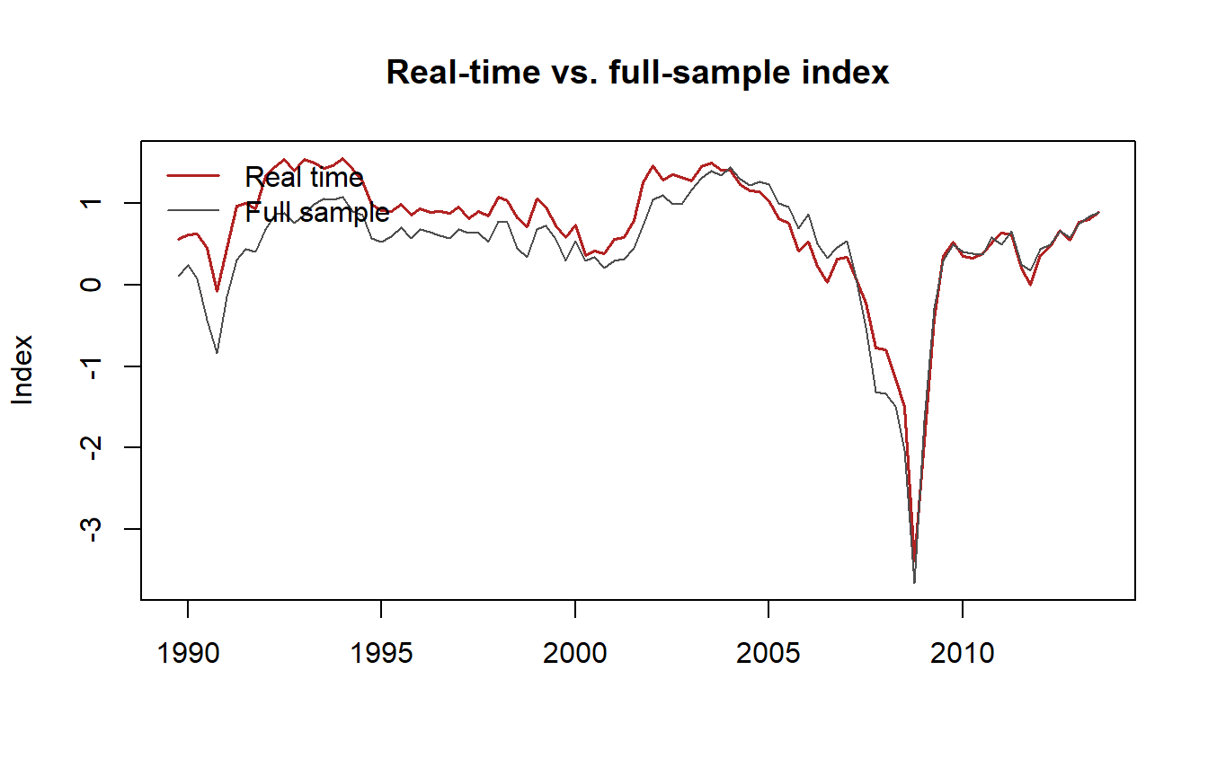

cor(realtime$index, final)

## [1] 0.9346385

A correlation above 0.93 between a reading made in real time and its own fully revised counterpart is the case for the index as a monitoring tool. Someone watching it as it was published would have seen essentially the same signal as someone looking back at it today – including through 2008, where both series reach their most extreme reading in the same quarter, 2008 Q4. That is not automatic for a factor extracted from a drifting model, and it is what makes the index usable for the purpose it was built for.

Two deviations from the published replication code

Reproducing the paper required departing from the code published with it in two places, both of which are documented in the package:

• Lags of the state. The replication code never fills the lag blocks of the companion form of the state, so it predicts from \(B_{1,t}\) alone. That is invisible at \(p = 1\) and incorrect above it. fincond carries the blocks, which is why the results above are not bit-identical to what the published code returns at \(p = 4\).
• Missing values. The replication code replaces missing values by the sample mean throughout, so a series that starts in 1990 contributes a constant to the index for the twenty years before it exists. fincond instead drops a series from the periods it is missing in, so it contributes from the date it starts and not before. A mean is still substituted for the principal components the algorithm is initialised from, which need a complete matrix and only set a starting value.

References

Koop, G., & Korobilis, D. (2014). A new index of financial conditions. European Economic Review, 71, 101–116. https://doi.org/10.1016/j.euroecorev.2014.07.002

Raftery, A. E., Kárný, M., & Ettler, P. (2010). Online prediction under model uncertainty via dynamic model averaging: Application to a cold rolling mill. Technometrics, 52(1), 52–66. https://doi.org/10.1198/TECH.2009.08104

West, M., & Harrison, J. (1997). Bayesian forecasting and dynamic models (2nd ed.). New York: Springer.