Reproduction: Timmer, M. P., Dietzenbacher, E., Los, B., Stehrer, R., & De Vries, G. J. (2015). An illustrated user guide to the world input–output database: the case of global automotive production.

Data

Timmer et al. (2015) use the 2013 vintage of the world input-output database (WIOD). The following code downloads the data from the project’s website, unzips it and loads the resulting STATA file into R using the readstata13 package.¹

# Download WIOD 2013
download.file("http://www.wiod.org/protected3/data13/update_sep12/wiot/wiot_stata_sep12.zip",
              destfile = "wiod13.zip")

# Unzip the file
unzip("wiod13.zip")

# Read dta file
library(readstata13)
data <- read.dta13("wiot_full.dta")

Value added export ratios in 2004

Timmer et al. (2015) compare different data sets on international input-output tables by calculating value-added exports (VAX) for a series of countries in 2004. VAX is a popular indicator, which measures a contry’s domestic value added embodied in final expenditures abroad.

In order to calculate VAX the Leontief decomposition is employed. In R this composition is implemented in the decompr package. The function decomp requires several input arguments: intermediate demand, final demand, a vector of country, a vector of industry and a vector of final outputs. The following code chunks can be used to obtain them.

# Load data manipulation packages
library(dplyr)
library(tidyr)

temp <- data %>%
  # Only use values for 2004
  filter(year == 2004) %>%
  # Sort by country and industry
  arrange(row_country, col_country, row_item, col_item) %>%
  # Rename the industry and demand codes
  mutate(row_item = as.character(row_item),
         col_item = as.character(col_item),
         row_item = ifelse(nchar(row_item) == 2, row_item, paste("0", row_item, sep = "")),
         col_item = ifelse(nchar(col_item) == 2, col_item, paste("0", col_item, sep = "")))

# Extract country names
countries <- unique(temp$col_country)

# Codes for intermediate industries
industries <- as.character(1:35)
industries <- ifelse(nchar(industries) == 2, industries, paste("0", industries, sep = ""))

# Codes for final demand
demand <- as.character(c(37, 38, 39, 41, 42))

The intermediate demand table is calculated by

# Intermediate demand
interm <- temp %>%
  filter(row_country %in% countries,
         row_item %in% industries,
         col_country %in% countries,
         col_item %in% industries) %>%
  mutate(col_country = paste(col_country, col_item, sep = "_")) %>%
  select(-col_item) %>%
  spread(col_country, value)

# Drop first three columns
interm <- interm[,-(1:3)]

Final demadn is obtained with

# Final demand
final <- temp %>%
  filter(row_country %in% countries,
         row_item %in% industries,
         col_country %in% countries,
         col_item %in% demand) %>%
  mutate(col_country = paste(col_country, col_item, sep = "_")) %>%
  select(-col_item) %>%
  spread(col_country, value)

# Drop first three columns
final <- final[, -(1:3)]

The elements of the final output vector are constructed as the sum of each row of the input-output table.

# Output
output <- temp %>%
  filter(row_country %in% countries,
         row_item %in% industries) %>%
  group_by(row_country, row_item) %>%
  summarise(value = sum(value)) %>%
  ungroup()

output <- output$value

Once the required tables have been created, they can be used as input for the Leontief decomposition. Note that by default decomp sets post = "exports", but in the context of this example post = final_demand is required.

library(decompr)

leon <- decomp(x = interm,
               y = final,
               k = countries,
               i = industries,
               o = output,
               method = "leontief",
               post = "final_demand")

VAX is calculated as domestic value added relative to gross exports. Using the WIOD gross exports are obtained as the sum over each row of the table, where values corresponding to domestic intermediate and final demand are omitted.

# Gross Exports
gross_exp <- temp %>%
  filter(row_country %in% countries,
         row_item %in% industries,
         col_country %in% countries,
         col_item %in% c(industries, demand)) %>%
  filter(row_country != col_country) %>%
  group_by(row_country) %>%
  summarise(exports = sum(value)) %>%
  ungroup()

Merging the results of the Leontief decomposition and gross exports per country allows to calculate value added exports:

# VAX ratio
vax <- leon %>%
  filter(Source_Country != Importing_Country) %>%
  group_by(Source_Country) %>%
  summarise(vax = sum(Final_Demand))%>%
  ungroup() %>%
  mutate(row_country = as.character(Source_Country)) %>%
  select(-Source_Country) %>%
  full_join(gross_exp, by = "row_country") %>%
  mutate(vax = vax / exports) %>%
  select(row_country, vax) %>%
  arrange(vax)

# Order observations by using factor
vax$row_country <- factor(vax$row_country, levels = vax$row_country)

The result can be plotted. The folling graph reproduces figure 2 in Timmer et al. (2015).

library(ggplot2)

ggplot(vax, aes(x = row_country, y = vax, colour = "a")) +
  geom_point(show.legend = FALSE) +
  scale_y_continuous(labels = scales::percent_format(accuracy = 1)) +
  scale_colour_brewer(palette = "Set1") +
  theme_classic() +
  theme(axis.text.x = element_text(angle = 90),
        axis.title = element_blank()) +
  labs(title = "Value Added Exports Ratios in 2004",
       subtitle = "VAX ratio",
       caption = "Source: WIOD.")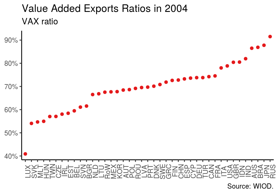

To be continued…

References

Garbuszus, J. M. & Jeworutzki, S. (2018). readstata13: Import ‘Stata’ Data Files. R package version 0.9.2. https://CRAN.R-project.org/package=readstata13

Quast, B. A. and V. Kummritz (2015). decompr: Global Value Chain decomposition in R. CTEI Working Papers, 1.

Timmer, M. P., Dietzenbacher, E., Los, B., Stehrer, R., & de Vries, G. J. (2015). An Illustrated User Guide to the World Input–Output Database: the Case of Global Automotive Production. Review of International Economics, 23(3), 575–605. https://doi.org/10.1111/roie.12178