Reproduction: Sheperd, B. (2016). The gravity model of international trade: A user guide.
with tags gravity trade r -The updated paper and dataset can be downloaded from UNESCAP.
Load libraries and read data
library(AER)
library(dplyr)
library(foreign)
library(ggplot2)
library(lmtest)
library(multiwayvcov)
library(sampleSelection)

data <- read.dta("servicesdataset_2016.dta")
Correlations
Table 1
data <- data %>%
  mutate(ln_trade = log(trade),
         ln_distance = log(dist),
         ln_gdp_exp = log(gdp_exp),
         ln_gdp_imp = log(gdp_imp))

cor.data <- data %>%
  filter(sector == "SER") %>%
  select(ln_trade, ln_gdp_exp, ln_gdp_imp, ln_distance) %>%
  na.omit %>%
  filter(ln_trade > -Inf)

round(cor(cor.data), 4)
## ln_trade ln_gdp_exp ln_gdp_imp ln_distance
## ln_trade 1.0000 0.3643 0.3731 -0.2648
## ln_gdp_exp 0.3643 1.0000 -0.3103 0.0518
## ln_gdp_imp 0.3731 -0.3103 1.0000 0.0431
## ln_distance -0.2648 0.0518 0.0431 1.0000Graphics
Prepare data
data <- data %>%
  mutate(ln_gdp_both = log(gdp_exp*gdp_imp))

plot.data <- data %>%
  filter(sector == "SER") %>%
  select(ln_gdp_both, ln_trade, ln_distance) %>%
  na.omit %>% filter(ln_trade > -Inf)
Figure 1
figure1 <- ggplot(plot.data, aes(x = ln_gdp_both, y = ln_trade)) +
  geom_point() +
  geom_smooth(se = FALSE, method = "lm") +
  scale_x_continuous(limits = c(40, 60)) +
  scale_y_continuous(limits = c(-7, 11))

figure1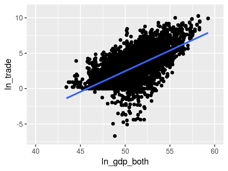
Figure 2
figure2 <- ggplot(plot.data, aes(x = ln_distance, y = ln_trade)) +
  geom_point() +
  geom_smooth(se = FALSE, method = "lm") +
  scale_x_continuous(limits = c(2, 10)) +
  scale_y_continuous(limits = c(-7, 11))

figure2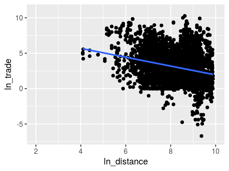
Table 2
data.table.02 <- data %>% filter(sector == "SER") %>%
  select(ln_trade, ln_gdp_exp, ln_gdp_imp, ln_distance, contig,
         comlang_off, colony, comcol, dist) %>%
  na.omit %>% filter(ln_trade != -Inf)

lm.table.02 <- lm(ln_trade ~ ln_gdp_exp + ln_gdp_imp + ln_distance +
                    contig + comlang_off + colony + comcol,
                  data = data.table.02)

summary(lm.table.02)
##
## Call:
## lm(formula = ln_trade ~ ln_gdp_exp + ln_gdp_imp + ln_distance +
## contig + comlang_off + colony + comcol, data = data.table.02)
##
## Residuals:
## Min 1Q Median 3Q Max
## -7.5085 -0.9359 0.0575 1.0070 5.8522
##
## Coefficients:
## Estimate Std. Error t value Pr(>|t|)
## (Intercept) -22.03706 0.54597 -40.363 <2e-16 ***
## ln_gdp_exp 0.60117 0.01252 48.002 <2e-16 ***
## ln_gdp_imp 0.61761 0.01267 48.730 <2e-16 ***
## ln_distance -0.73851 0.02809 -26.294 <2e-16 ***
## contig 0.39895 0.15896 2.510 0.0121 *
## comlang_off 0.88613 0.08969 9.879 <2e-16 ***
## colony 1.20297 0.11388 10.564 <2e-16 ***
## comcol -0.02451 0.19831 -0.124 0.9017
## ---
## Signif. codes: 0 '***' 0.001 '**' 0.01 '*' 0.05 '.' 0.1 ' ' 1
##
## Residual standard error: 1.528 on 3876 degrees of freedom
## Multiple R-squared: 0.5431, Adjusted R-squared: 0.5422
## F-statistic: 658.1 on 7 and 3876 DF, p-value: < 2.2e-16vcov.02 <- cluster.vcov(lm.table.02, ~ dist)
coeftest(lm.table.02, vcov. = vcov.02)##
## t test of coefficients:
##
## Estimate Std. Error t value Pr(>|t|)
## (Intercept) -22.037061 0.671738 -32.8060 < 2e-16 ***
## ln_gdp_exp 0.601167 0.013221 45.4710 < 2e-16 ***
## ln_gdp_imp 0.617606 0.014267 43.2904 < 2e-16 ***
## ln_distance -0.738515 0.035360 -20.8856 < 2e-16 ***
## contig 0.398952 0.182928 2.1809 0.02925 *
## comlang_off 0.886133 0.099308 8.9231 < 2e-16 ***
## colony 1.202965 0.120197 10.0083 < 2e-16 ***
## comcol -0.024507 0.201819 -0.1214 0.90336
## ---
## Signif. codes: 0 '***' 0.001 '**' 0.01 '*' 0.05 '.' 0.1 ' ' 1If found the code for the clustered standard errors here.
Table 3
Not sure how to do that in R.
Table 4
lm.ols.ncult <- lm(ln_trade ~ ln_gdp_exp + ln_gdp_imp + ln_distance,
                   data = data.table.02)

waldtest(lm.ols.ncult, lm.table.02, vcov = vcov.02)
## Wald test
##
## Model 1: ln_trade ~ ln_gdp_exp + ln_gdp_imp + ln_distance
## Model 2: ln_trade ~ ln_gdp_exp + ln_gdp_imp + ln_distance + contig + comlang_off +
## colony + comcol
## Res.Df Df F Pr(>F)
## 1 3880
## 2 3876 4 100.16 < 2.2e-16 ***
## ---
## Signif. codes: 0 '***' 0.001 '**' 0.01 '*' 0.05 '.' 0.1 ' ' 1Table 5
data.table.05 <- data %>% filter(sector == "SER") %>%
  select(ln_trade, etcr_exp, etcr_imp, ln_gdp_exp, ln_gdp_imp, ln_distance, contig,
         comlang_off, colony, comcol, dist) %>%
  na.omit %>% filter(ln_trade != -Inf)

lm.table.05 <- lm(ln_trade ~ etcr_exp + etcr_imp + ln_gdp_exp + ln_gdp_imp +
                    ln_distance + contig + comlang_off + colony + comcol,
                  data = data.table.05)

vcov.05 <- cluster.vcov(lm.table.05, ~ dist)
coeftest(lm.table.05, vcov. = vcov.05)
##
## t test of coefficients:
##
## Estimate Std. Error t value Pr(>|t|)
## (Intercept) -27.110231 1.799003 -15.0696 < 2.2e-16 ***
## etcr_exp -0.360526 0.091040 -3.9601 8.154e-05 ***
## etcr_imp -0.372200 0.079639 -4.6736 3.468e-06 ***
## ln_gdp_exp 0.773685 0.034945 22.1400 < 2.2e-16 ***
## ln_gdp_imp 0.822348 0.034943 23.5339 < 2.2e-16 ***
## ln_distance -1.114939 0.062647 -17.7970 < 2.2e-16 ***
## contig -0.557999 0.245254 -2.2752 0.02316 *
## comlang_off 1.378263 0.209096 6.5915 7.858e-11 ***
## colony 0.177106 0.207763 0.8524 0.39422
## ---
## Signif. codes: 0 '***' 0.001 '**' 0.01 '*' 0.05 '.' 0.1 ' ' 1Table 6
data.table.06 <- data %>%
  filter(sector == "SER") %>%
  select(ln_trade, ln_distance, contig, comlang_off, colony,
         comcol, dist, exp, imp) %>%
  na.omit %>%
  filter(ln_trade != -Inf)

lm.table.06 <- lm(ln_trade ~ ln_distance + contig + comlang_off +
                    colony + comcol + exp + imp,
                  data = data.table.06)

vcov.06 <- cluster.vcov(lm.table.06, ~ dist)
coeftest(lm.table.06, vcov. = vcov.06)
##
## t test of coefficients:
##
## Estimate Std. Error t value Pr(>|t|)
## (Intercept) 6.59190484 0.90904034 7.2515 4.975e-13 ***
## ln_distance -1.01476740 0.04692188 -21.6267 < 2.2e-16 ***
## contig 0.23559097 0.20218504 1.1652 0.2440017
## comlang_off 0.39823504 0.09369219 4.2505 2.185e-05 ***
## colony 1.17362816 0.11599078 10.1183 < 2.2e-16 ***
## comcol -0.08862510 0.25844959 -0.3429 0.7316848
## expAFG -0.33862711 0.53086888 -0.6379 0.5235948
## expAGO 2.01064971 0.68592191 2.9313 0.0033956 **
## expAIA -0.84611895 0.61167757 -1.3833 0.1666619
## expALB -1.75333683 0.81322640 -2.1560 0.0311446 *
## [ reached getOption("max.print") -- omitted 395 rows ]
## ---
## Signif. codes: 0 '***' 0.001 '**' 0.01 '*' 0.05 '.' 0.1 ' ' 1Table 7
Not sure yet
data.table.07 <- data %>%
  filter(sector == "SER") %>%
  select(ln_trade, ln_distance, contig, comlang_off, colony,
         comcol, dist, exp, imp) %>%
  na.omit %>%
  filter(ln_trade != -Inf)

lm.table.07 <- lm(ln_trade ~ ln_distance + contig + comlang_off +
                    colony + comcol + exp + imp,
                  data = data.table.07)

vcov.07 <- cluster.vcov(lm.table.07, ~ dist)
coeftest(lm.table.07, vcov. = vcov.07)
##
## t test of coefficients:
##
## Estimate Std. Error t value Pr(>|t|)
## (Intercept) 6.59190484 0.90904034 7.2515 4.975e-13 ***
## ln_distance -1.01476740 0.04692188 -21.6267 < 2.2e-16 ***
## contig 0.23559097 0.20218504 1.1652 0.2440017
## comlang_off 0.39823504 0.09369219 4.2505 2.185e-05 ***
## colony 1.17362816 0.11599078 10.1183 < 2.2e-16 ***
## comcol -0.08862510 0.25844959 -0.3429 0.7316848
## expAFG -0.33862711 0.53086888 -0.6379 0.5235948
## expAGO 2.01064971 0.68592191 2.9313 0.0033956 **
## expAIA -0.84611895 0.61167757 -1.3833 0.1666619
## expALB -1.75333683 0.81322640 -2.1560 0.0311446 *
## [ reached getOption("max.print") -- omitted 395 rows ]
## ---
## Signif. codes: 0 '***' 0.001 '**' 0.01 '*' 0.05 '.' 0.1 ' ' 1Table 8
data.table.08 <- data %>%
  filter(sector == "SER") %>%
  select(ln_trade, etcr_exp, etcr_imp, ln_distance, contig,
         comlang_off, colony, comcol, dist, exp, imp) %>%
  mutate(etcr_both = etcr_exp*etcr_imp) %>%
  na.omit %>%
  filter(ln_trade != -Inf)

lm.table.08 <- lm(ln_trade ~ etcr_both + ln_distance + contig +
                    comlang_off + colony + comcol + exp + imp,
                  data = data.table.08)

vcov.08 <- cluster.vcov(lm.table.08, ~ dist)
coeftest(lm.table.08, vcov. = vcov.08)
##
## t test of coefficients:
##
## Estimate Std. Error t value Pr(>|t|)
## (Intercept) 12.790243 1.405801 9.0982 < 2.2e-16 ***
## etcr_both -0.304270 0.091759 -3.3160 0.0009571 ***
## ln_distance -0.897964 0.107326 -8.3667 2.873e-16 ***
## contig 0.325120 0.264871 1.2275 0.2200308
## comlang_off 0.208773 0.191935 1.0877 0.2770640
## colony 0.461365 0.272334 1.6941 0.0906575 .
## expAUT -0.882587 0.408199 -2.1622 0.0309212 *
## expBEL 0.316488 0.429214 0.7374 0.4611299
## expCAN 0.434073 0.332142 1.3069 0.1916496
## expCHE 1.345860 0.447139 3.0099 0.0027004 **
## [ reached getOption("max.print") -- omitted 54 rows ]
## ---
## Signif. codes: 0 '***' 0.001 '**' 0.01 '*' 0.05 '.' 0.1 ' ' 1Table 9
data.table.09 <- data %>%
  filter(sector == "SER") %>%
  select(ln_trade, ln_distance, dist, exp, imp) %>%
  na.omit %>% filter(ln_trade != -Inf)

lm.table.09 <- lm(ln_trade ~ ln_distance + exp + imp,
                  data = data.table.09)

vcov.09 <- cluster.vcov(lm.table.09, ~ dist)
coeftest(lm.table.09, vcov. = vcov.09)
##
## t test of coefficients:
##
## Estimate Std. Error t value Pr(>|t|)
## (Intercept) 8.3121731 1.2891856 6.4476 1.280e-10 ***
## ln_distance -1.1283121 0.0462662 -24.3874 < 2.2e-16 ***
## expAFG -0.6754424 0.6341010 -1.0652 0.2868548
## expAGO 1.9197110 0.8465990 2.2676 0.0234124 *
## expAIA -0.3117572 0.5766871 -0.5406 0.5888150
## expALB -2.1442015 0.8997349 -2.3831 0.0172144 *
## expAND -1.1497718 1.0257781 -1.1209 0.2624110
## expANT 2.2124493 0.6912184 3.2008 0.0013818 **
## expARE 3.3236739 0.5783296 5.7470 9.800e-09 ***
## expARG 1.6644259 0.6427583 2.5895 0.0096482 **
## [ reached getOption("max.print") -- omitted 391 rows ]
## ---
## Signif. codes: 0 '***' 0.001 '**' 0.01 '*' 0.05 '.' 0.1 ' ' 1Table 10
data.table.10 <- data %>%
  select(ln_trade, ln_distance, dist, exp, imp, sector, ln_gdp_exp, ln_gdp_imp)

temp1 <- data.table.10 %>%
  group_by(exp, sector) %>%
  summarise(temp1 = mean(ln_distance, na.rm = TRUE))

temp2 <- data.table.10 %>%
  group_by(imp, sector) %>%
  summarise(temp2 = mean(ln_distance, na.rm = TRUE))

temp3 <- data.table.10 %>%
  group_by(sector) %>%
  summarise(temp3 = sum(ln_distance, na.rm = TRUE))

data.table.10 <- left_join(data.table.10, temp1)
data.table.10 <- left_join(data.table.10, temp2)
data.table.10 <- left_join(data.table.10, temp3)

data.table.10 <- data.table.10 %>%
  mutate(ln_distance_star = ln_distance - temp1 - temp2 + (1/218^2)*temp3)

data.table.10 <- filter(data.table.10, sector == "SER") %>%
  select(ln_trade, ln_distance_star, ln_gdp_exp, ln_gdp_imp, dist) %>%
  na.omit %>%
  filter(ln_trade != -Inf)

lm.table.10 <- lm(ln_trade ~ ln_distance_star + ln_gdp_exp + ln_gdp_imp,
                  data = data.table.10)

vcov.10 <- cluster.vcov(lm.table.10, ~ dist)
coeftest(lm.table.10, vcov. = vcov.10)
##
## t test of coefficients:
##
## Estimate Std. Error t value Pr(>|t|)
## (Intercept) -35.014552 0.703602 -49.765 < 2.2e-16 ***
## ln_distance_star -1.142375 0.050619 -22.568 < 2.2e-16 ***
## ln_gdp_exp 0.572658 0.013149 43.551 < 2.2e-16 ***
## ln_gdp_imp 0.588375 0.014007 42.004 < 2.2e-16 ***
## ---
## Signif. codes: 0 '***' 0.001 '**' 0.01 '*' 0.05 '.' 0.1 ' ' 1Table 11a
data.table.11 <- data %>%
  mutate(ln_lat_exp = log(abs(lat_exp)),
         ln_lat_imp = log(abs(lat_imp))) %>%
  select(ln_trade, etcr_exp, etcr_imp, ln_lat_exp, ln_lat_imp, ln_gdp_exp,
         ln_gdp_imp, ln_distance, contig, comlang_off, colony, comcol, dist) %>%
  na.omit %>%
  filter(ln_trade != -Inf)

iv.t11a <- ivreg(etcr_exp ~ ln_gdp_exp + ln_gdp_imp + ln_distance + contig +
                   comlang_off + colony + ln_lat_exp + ln_lat_imp,
                 data = data.table.11)

vcov.11a <- cluster.vcov(iv.t11a, ~ dist)
coeftest(iv.t11a, vcov. = vcov.11a)
##
## t test of coefficients:
##
## Estimate Std. Error t value Pr(>|t|)
## (Intercept) 15.671204 1.054823 14.8567 < 2.2e-16 ***
## ln_gdp_exp -0.168561 0.010199 -16.5266 < 2.2e-16 ***
## ln_gdp_imp 0.011711 0.015874 0.7377 0.46072
## ln_distance -0.155711 0.024894 -6.2548 4.449e-10 ***
## contig -0.119582 0.115226 -1.0378 0.29943
## comlang_off -0.189698 0.105539 -1.7974 0.07235 .
## colony 0.031553 0.149608 0.2109 0.83298
## ln_lat_exp -1.924733 0.101698 -18.9260 < 2.2e-16 ***
## ln_lat_imp -0.158599 0.119829 -1.3235 0.18574
## ---
## Signif. codes: 0 '***' 0.001 '**' 0.01 '*' 0.05 '.' 0.1 ' ' 1Table 11b
iv.t11b <- ivreg(etcr_imp ~ ln_gdp_exp + ln_gdp_imp + ln_distance + contig +
                   comlang_off + colony + ln_lat_exp + ln_lat_imp,
                 data = data.table.11)

vcov.11b <- cluster.vcov(iv.t11b, ~ dist)
coeftest(iv.t11b, vcov. = vcov.11b)
##
## t test of coefficients:
##
## Estimate Std. Error t value Pr(>|t|)
## (Intercept) 15.767842 1.017276 15.5001 < 2.2e-16 ***
## ln_gdp_exp 0.006375 0.015536 0.4103 0.68159
## ln_gdp_imp -0.179440 0.010476 -17.1293 < 2.2e-16 ***
## ln_distance -0.127436 0.024210 -5.2639 1.493e-07 ***
## contig -0.066829 0.114022 -0.5861 0.55784
## comlang_off -0.199469 0.110249 -1.8093 0.07049 .
## colony 0.024146 0.154112 0.1567 0.87551
## ln_lat_exp -0.122387 0.113011 -1.0830 0.27890
## ln_lat_imp -1.934644 0.109432 -17.6790 < 2.2e-16 ***
## ---
## Signif. codes: 0 '***' 0.001 '**' 0.01 '*' 0.05 '.' 0.1 ' ' 1Table 11c
iv.t11c <- ivreg(ln_trade ~ etcr_exp + etcr_imp + ln_gdp_exp + ln_gdp_imp +
                   ln_distance + contig + comlang_off + colony |
                   ln_lat_exp + ln_lat_imp + ln_gdp_exp + ln_gdp_imp +
                   ln_distance + contig + comlang_off + colony,
                 data = data.table.11)

vcov.11c <- cluster.vcov(iv.t11c, ~ dist)
coeftest(iv.t11c, vcov. = vcov.11c)
##
## t test of coefficients:
##
## Estimate Std. Error t value Pr(>|t|)
## (Intercept) -20.427808 1.849596 -11.0445 < 2.2e-16 ***
## etcr_exp -0.542214 0.150151 -3.6111 0.000309 ***
## etcr_imp -0.467479 0.108044 -4.3267 1.555e-05 ***
## ln_gdp_exp 0.618591 0.033052 18.7157 < 2.2e-16 ***
## ln_gdp_imp 0.698783 0.033822 20.6607 < 2.2e-16 ***
## ln_distance -1.149847 0.065328 -17.6011 < 2.2e-16 ***
## contig -0.535280 0.285332 -1.8760 0.060738 .
## comlang_off 1.128319 0.244922 4.6069 4.230e-06 ***
## colony -0.025328 0.294506 -0.0860 0.931470
## ---
## Signif. codes: 0 '***' 0.001 '**' 0.01 '*' 0.05 '.' 0.1 ' ' 1The coefficients are the same, but the clustered standard errors are not. I am not sure, where this comes from.
Table 12
data.table.12 <- data %>%
  filter(sector == "SER") %>%
  select(trade, ln_distance, contig, comlang_off, colony,
         comcol, exp, imp, dist) %>%
  na.omit

est.table.12 <- glm(trade ~ ln_distance + contig + comlang_off + colony +
                      comcol + exp + imp, family = "quasipoisson",
                    data = data.table.12)

vcov.12 <- cluster.vcov(est.table.12, ~ dist)
coeftest(est.table.12, vcov. = vcov.12)
##
## z test of coefficients:
##
## Estimate Std. Error z value Pr(>|z|)
## (Intercept) 3.621280 1.650720 2.1938 0.0282528 *
## ln_distance -0.557670 0.049962 -11.1618 < 2.2e-16 ***
## contig 0.220584 0.172437 1.2792 0.2008216
## comlang_off 0.459272 0.121251 3.7878 0.0001520 ***
## colony 0.142065 0.119081 1.1930 0.2328656
## comcol -0.552796 0.386683 -1.4296 0.1528359
## expAFG -1.325194 0.891621 -1.4863 0.1372064
## expAGO 2.469760 0.824305 2.9962 0.0027339 **
## expAIA -2.196090 0.823901 -2.6655 0.0076879 **
## expALB -3.260660 1.149748 -2.8360 0.0045686 **
## [ reached getOption("max.print") -- omitted 408 rows ]
## ---
## Signif. codes: 0 '***' 0.001 '**' 0.01 '*' 0.05 '.' 0.1 ' ' 1The coefficients are the same, but the clustered standard errors are not. I am not sure, where this comes from.
Table 13
data <- mutate(data, ent_cost_both = ent_cost_exp*ent_cost_imp)

data.table.13 <- data %>%
  filter(sector == "SER") %>%
  select(ln_trade, ln_distance, contig, comlang_off, colony, comcol,
         exp, imp, ent_cost_both, dist) %>%
  na.omit %>%
  mutate(select = as.numeric(ln_trade != -Inf))

data.table.13[!data.table.13[,"select"], "ln_trade"] <- NA
data.table.13[, "exp"] <- factor(data.table.13[, "exp"])
data.table.13[, "imp"] <- factor(data.table.13[, "imp"])

# Deviates from the 1st-step results in the paper
summary(probit(select ~ ln_distance + contig + comlang_off + colony +
                 comcol + ent_cost_both + exp + imp,
               data = data.table.13))
## --------------------------------------------
## Probit binary choice model/Maximum Likelihood estimation
## Newton-Raphson maximisation, 15 iterations
## Return code 2: successive function values within tolerance limit
## Log-Likelihood: -1304.324
## Model: Y == '1' in contrary to '0'
## 5164 observations (1681 'negative' and 3483 'positive') and 337 free parameters (df = 4827)
## Estimates:
## Estimate Std. error t value Pr(> t)
## (Intercept) 1.1898e+00 9.3780e-01 1.2688 0.2045298
## ln_distance -6.5453e-01 7.0904e-02 -9.2313 < 2.2e-16 ***
## contig 9.1742e-01 3.7431e-01 2.4510 0.0142476 *
## comlang_off 4.1025e-01 1.4029e-01 2.9243 0.0034520 **
## colony 8.2522e-01 2.0629e-01 4.0002 6.328e-05 ***
## comcol 1.2328e-01 2.2706e-01 0.5429 0.5871839
## ent_cost_both -2.1996e-01 2.4470e-01 -0.8989 0.3686997
## expAGO 1.5698e+00 6.6724e-01 2.3527 0.0186387 *
## expALB -1.1498e+00 6.1461e-01 -1.8708 0.0613727 .
## expARE 2.9294e+00 8.9968e-01 3.2561 0.0011295 **
## [ reached getOption("max.print") -- omitted 327 rows ]
## ---
## Signif. codes: 0 '***' 0.001 '**' 0.01 '*' 0.05 '.' 0.1 ' ' 1
## Significance test:
## chi2(336) = 3907.932 (p=0)
## --------------------------------------------# est.table.13 <- selection(select ~ ln_distance + contig + comlang_off + colony + comcol + ent_cost_both + exp + imp, ln_trade ~ ln_distance + contig + comlang_off + colony + comcol + exp + imp, data = data.table.13)
# Produces an error
#vcov.13 <- cluster.vcov(est.table.13, ~ dist)
#coeftest(est.table.13, vcov. = vcov.13)