Chapter 11: Monte Carlo Integration
Exercise 11.2: Drawing frmm standard distributions
# Sample size
n1 <- 10L
n2 <- 100L
n3 <- 100000L
# We use integers as indicated by the "L" at the end of the number.
# This only makes the results look nicer

# Reset random number generator for reproducibilty
set.seed(123456)
Uniform
The standard specification of R’s random number generator (RNG) runif is min = 0 and max = 1, which is exactly what we need. So we only have to specify the number of draws.
unif1 <- runif(n1)
unif2 <- runif(n2)
unif3 <- runif(n3)

result <- data.frame(size = c(n1, n2, n3),
                     mean = c(mean(unif1), mean(unif2), mean(unif3)),
                     sd = c(sd(unif1), sd(unif2), sd(unif3)))

result
## size mean sd
## 1 10 0.4630601 0.2979562
## 2 100 0.4929105 0.3095004
## 3 100000 0.4990746 0.2891135Standard normal
The standard specification of R’s RNG for the normal distribution rnorm is mean = 0 and sd = 1, which is by definition a standard normal distribution. So we only have to specify the number of draws.
norm1 <- rnorm(n1)
norm2 <- rnorm(n2)
norm3 <- rnorm(n3)

result <- data.frame(size = c(n1, n2, n3),
                     mean = c(mean(norm1), mean(norm2), mean(norm3)),
                     sd = c(sd(norm1), sd(norm2), sd(norm3)))

result
## size mean sd
## 1 10 -0.149059541 1.149290
## 2 100 -0.076840784 1.090117
## 3 100000 0.001551597 1.001076Student t(3)
t1 <- rt(n1, df = 3)
t2 <- rt(n2, df = 3)
t3 <- rt(n3, df = 3)

result <- data.frame(size = c(n1, n2, n3),
                     mean = c(mean(t1), mean(t2), mean(t3)),
                     sd = c(sd(t1), sd(t2), sd(t3)))

result
## size mean sd
## 1 10 0.523968595 1.427517
## 2 100 -0.100952189 1.361346
## 3 100000 -0.008228298 1.720145Beta(3,2)
beta1 <- rbeta(n1, shape1 = 3, shape2 = 2)
beta2 <- rbeta(n2, shape1 = 3, shape2 = 2)
beta3 <- rbeta(n3, shape1 = 3, shape2 = 2)

result <- data.frame(size = c(n1, n2, n3),
                     mean = c(mean(beta1), mean(beta2), mean(beta3)),
                     sd = c(sd(beta1), sd(beta2), sd(beta3)))

result
## size mean sd
## 1 10 0.6460647 0.1927849
## 2 100 0.5902536 0.1927114
## 3 100000 0.5995364 0.1999195Exponential(5)
To show the equivalence of the exponential(5) distribution and the G(1, 5) distribution, we reset the RNG before we draw from the respective distribution.
Also note that \(rexp\) requires a slightly different input than the mean as described in the textbook. Rather, we have to specify the rate of the distribution, which is defined as 1 / mean.
set.seed(987654) # Reset RNG

exp1 <- rexp(n1, rate = 1 / 5)
exp2 <- rexp(n2, rate = 1 / 5)
exp3 <- rexp(n3, rate = 1 / 5)

result <- data.frame(size = c(n1, n2, n3),
                     mean = c(mean(exp1), mean(exp2), mean(exp3)),
                     sd = c(sd(exp1), sd(exp2), sd(exp3)))

result
## size mean sd
## 1 10 6.066529 4.766100
## 2 100 5.567845 5.514212
## 3 100000 4.991803 4.994150Gamma(1, 5)
set.seed(987654) # Reset RNG

gamma_exp1 <- rgamma(n1, shape = 1, scale = 5)
gamma_exp2 <- rgamma(n2, shape = 1, scale = 5)
gamma_exp3 <- rgamma(n3, shape = 1, scale = 5)

result <- data.frame(size = c(n1, n2, n3),
                     mean = c(mean(gamma_exp1), mean(gamma_exp2), mean(gamma_exp3)),
                     sd = c(sd(gamma_exp1), sd(gamma_exp2), sd(gamma_exp3)))

result
## size mean sd
## 1 10 4.439433 2.772297
## 2 100 4.856169 4.603918
## 3 100000 4.995174 5.002952Although numerically not the same, it can be shown that the two approaches are equivalent by using one million draws and plotting their histograms:
library(ggplot2)

# Exponential distribution
set.seed(987654) # Reset RNG
exp4 <- data.frame(var = "Exponential(5)", value = rexp(10^6, rate = 1 / 5))

# Gamma distribution
set.seed(987654) # Reset RNG
gamma_exp4 <- data.frame(var = "Gamma(1, 5)", value = rgamma(10^6, shape = 1, scale = 5))

temp <- rbind(exp4, gamma_exp4)

ggplot(temp, aes(x = value, fill = var)) +
  geom_histogram(position = "dodge")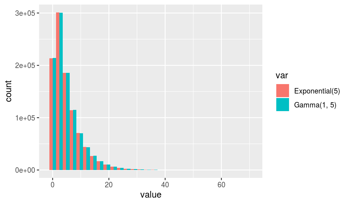
Note that you could also specify the \(rate\) argument in \(rgamma\) to obtain the same result. In this case rate is defined as 1 / scale.
set.seed(987654) # Reset RNG

gamma_exp1 <- rgamma(n1, shape = 1, rate = 1 / 5)
gamma_exp2 <- rgamma(n2, shape = 1, rate = 1 / 5)
gamma_exp3 <- rgamma(n3, shape = 1, rate = 1 / 5)

result <- data.frame(size = c(n1, n2, n3),
                     mean = c(mean(gamma_exp1), mean(gamma_exp2), mean(gamma_exp3)),
                     sd = c(sd(gamma_exp1), sd(gamma_exp2), sd(gamma_exp3)))

result
## size mean sd
## 1 10 4.439433 2.772297
## 2 100 4.856169 4.603918
## 3 100000 4.995174 5.002952The rate argument can be very handy if you want to draw from a inverse gamma distribution, which is often the case in Gibbs sampling.
Chi-squared(2)
Again, to show the equivalence of the \(\chi^{2}(5)\) distribution and the \(G(1, 5)\) distribution, we reset the RNG before we draw from the respective distribution.
set.seed(987654) # Reset RNG

chisq1 <- rchisq(n1, 3)
chisq2 <- rchisq(n2, 3)
chisq3 <- rchisq(n3, 3)

result <- data.frame(size = c(n1, n2, n3),
                     mean = c(mean(chisq1), mean(chisq2), mean(chisq3)),
                     sd = c(sd(chisq1), sd(chisq2), sd(chisq3)))

result
## size mean sd
## 1 10 2.563593 1.633190
## 2 100 3.050965 2.245561
## 3 100000 3.006940 2.452734Gamma(3/2, 2)
set.seed(987654) # Reset RNG

gamma_chi1 <- rgamma(n1, shape = 3 / 2, scale = 2)
gamma_chi2 <- rgamma(n2, shape = 3 / 2, scale = 2)
gamma_chi3 <- rgamma(n3, shape = 3 / 2, scale = 2)

result <- data.frame(size = c(n1, n2, n3),
                     mean = c(mean(gamma_chi1), mean(gamma_chi2), mean(gamma_chi3)),
                     sd = c(sd(gamma_chi1), sd(gamma_chi2), sd(gamma_chi3)))

result
## size mean sd
## 1 10 2.563593 1.633190
## 2 100 3.050965 2.245561
## 3 100000 3.006940 2.452734In this case, the output of the two approaches is exaclty the same, which results from reseting the RNG seed.
Exercise 11.3: Monte Carlo integration in a regression problem
Generate artificial data set
set.seed(987654) # Reset RNG

n <- 100 # Number of observations

# Specify coefficients
beta1 <- 0
beta2 <- 1
h <- 1

# Generate random draws of explanatory variables
x <- runif(n)

# Generate random draws of errors
epsilon <- rnorm(n, 0, 1 / h)

# Calculate depended variable
y <- beta1 + beta2 * x + epsilon
y <- matrix(y) # Transform to matrix format for later

# Generate data matrix of regressors
x <- cbind(1, x)

# Number of regressors
k <- ncol(x)
Calculate posterior mean and standard deviation
Set priors
beta_mu_prior <- matrix(c(0, 1)) # Prior mean
beta_v_i_prior <- diag(1, k) # Prior covariance

v_prior <- 1 # Prior degrees of freedom
s2_prior <- 1 # Prior variance
Obtain posteriors
# OLS results
b_hat <- solve(crossprod(x)) %*% crossprod(x, y) # OLS estimate
v <- n - k # Degrees of freedom
s2 <- crossprod(y - x %*% b_hat) / v # sigma2
sse <- v * s2 # SSE

# beta posterior
beta_v_i_post <- solve(beta_v_i_prior + crossprod(x))
beta_mu_post <- beta_v_i_post %*% (beta_v_i_prior %*% beta_mu_prior + crossprod(x) %*% b_hat)


v_post <- v_prior + n

beta_diff <- b_hat - beta_mu_prior

vs_post <- as.numeric(v_prior * s2_prior + sse + crossprod(beta_diff, crossprod(x) %*% beta_v_i_post %*% beta_v_i_prior) %*% beta_diff)
s2_post <- vs_post / v_post
Posterior mean and standard deviation
beta_cov <- beta_v_i_post * vs_post / (v_post - k)
beta_sd <- sqrt(diag(beta_cov))

result <- data.frame(beta_mu = beta_mu_post,
                     beta_sd = beta_sd)
row.names(result) <- c("beta1", "beta2")

result
## beta_mu beta_sd
## beta1 0.03296222 0.1864333
## beta2 0.63769948 0.3337710Work in progress