Chapter 18: State Space and Unobserved Components Models
Exercise 18.1: The local level model
Data: US PCE inflation until 2015Q4
# Specify URL
url <- "https://web.ics.purdue.edu/~jltobias/second_edition/Chapter18/code_for_exercise_1/USPCE_2015Q4.csv"

# Load data
pce <- read.csv(url, header = FALSE, col.names = "pci")

# Log growth rates
pce <- diff(ts(log(pce), start = 1959, frequency = 4))

# Rescale
y <- matrix(pce * 100 * 4, 1)
tt <- ncol(y) # T
z <- diag(1, tt) # Data matrix
Estimation
Prior
a0 <- 5
b0 <- 100
Initial values
library(bvartools)
library(Matrix)

# Difference matrix
H <- diag(1, tt)
diag(H[2:tt, 1:(tt - 1)]) <- -1

# (Inverse) variance of the measeurement equation
sigma <- var(c(y))
sigma_i <- solve(sigma)
sigma_i <- kronecker(diag(1, tt), sigma_i)

# Inverse variance of the transition equation
q_i <- kronecker(diag(1, tt), 1 / 100)

# Inital state
tau0 <- matrix(y[1])

# Transform into sparse matrices so that function chan_jeliazkov can be used
z <- Matrix(z)
H <- Matrix(H)
sigma_i <- Matrix(sigma_i)
q_i <- Matrix(q_i)
Gibbs sampler
iterations <- 21000
burnin <- 1000

# Container for draws
draws_tau <- matrix(NA, tt, iterations - burnin)

for (draw in 1:iterations) {
  # Draw trend
  a <- chan_jeliazkov(y, z, sigma_i, H, q_i, tau0)

  # Draw measurement eq. variance
  u <- y - a[, -1]
  diag(sigma_i) <- rgamma(1, shape = 3 + tt / 2, rate = 2 + tcrossprod(u) / 2)

  # Draw transition eq. variance
  w <- a[, -1] - matrix(a0, 1, tt)
  w <- w %*% as.matrix(crossprod(H)) %*% t(w)
  diag(q_i) <- rgamma(1, shape = 3 + tt / 2, rate = 2 * .25^2 + w / 2)

  # Draw initial condition
  K_tau0 <- 1 / b0 + q_i[1, 1]
  mu_tau0 <- 1 / K_tau0 * (a0 / b0 + a[, 2] * q_i[1, 1])
  tau0 <- rnorm(1, mu_tau0, sqrt(1 / K_tau0))

  # Save draws
  if (draw > burnin) {
    draws_tau[, draw - burnin] <- a[, -1]
  }
}
Plot estimated prior mean of tau
tau <- apply(draws_tau, 1, mean) # Mean
tau <- cbind(c(y), tau) # Combine with original series
tau <- ts(tau, start = 1959, frequency = 4)

plot(tau, plot.type = "single", col = c("black", "red"),
     ylim = c(-15, 20), ylab = "")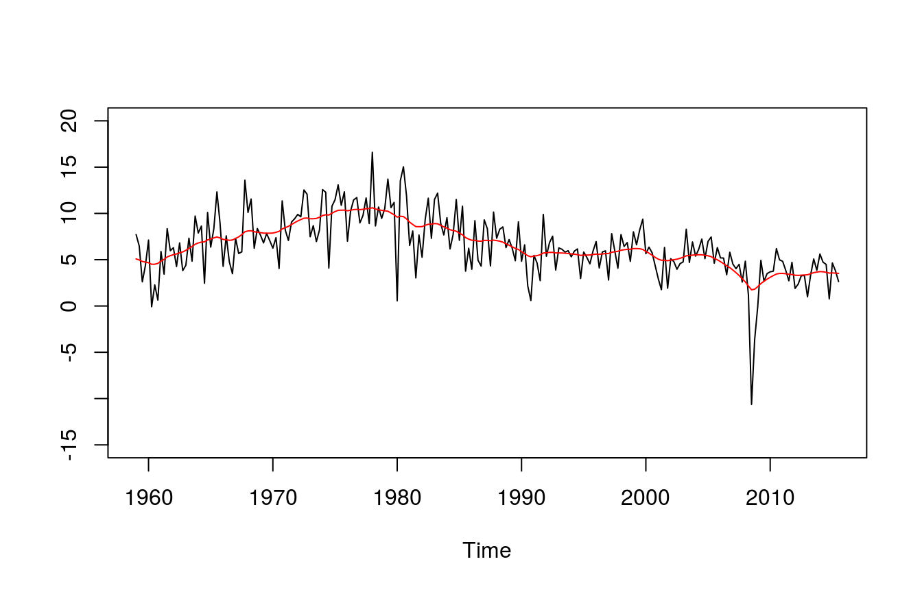
Exercise 18.2: Estimating the output gap
The approach follows Grant, A. L., & Chan, J. C. C. (2017). Reconciling output gaps: Unobserved components model and Hodrick-Prescott filter, Journal of Economic Dynamics and Control, 75, 114-121.
Data: US log GDP until 2015Q4
# Specify URL
url <- "https://web.ics.purdue.edu/~jltobias/second_edition/Chapter18/code_for_exercise_2/USGDP_2015Q4.csv"

# Download data
gdp <- read.csv(url, header = FALSE)[, 1]

y <- matrix(log(gdp) * 100) # Log GDP
p <- 2 # Lag of cyclical component
tt <- nrow(y) # T
Estimation
Priors
# Priors of phi
prior_phi_mu <- matrix(c(1.3, -.7))
prior_phi_v_i <- diag(1, p)

# Priors of gamma
prior_gamma_mu <- matrix(c(750, 750)) # Should be close to first value of the series
prior_gamma_v_i <- diag(1 / 100, p)

# Priors for sigma2_tau
prior_s_tau <- .01

# Priors for sigma2_c
prior_s_c_shape <- 3
prior_s_c_rate <- 2
Initial values
# X_gamma
x_gamma <- cbind(2:(tt + 1), -1:-tt)

# H_2
h2 <- diag(1, tt)
diag(h2[-1, -tt]) <- -2
diag(h2[-(1:2), -((tt - 1):tt)]) <- 1
h2h2 <- crossprod(h2)

# H_phi
h_phi <- diag(1, tt)
phi <- matrix(c(1.34, -.7))
for (i in 1:p) {
  diag(h_phi[-(1:i), -((tt - i):tt)]) <- -phi[i,]
}

# Inverse of sigma tau
s_tau_i <- 1 / .001

# Inverse of sigma c
s_c_i <- 1 / .5

# gamma
gamma <- t(rep(y[1], 2)) # Should be close to first value of the series
Gibbs sampler
iterations <- 11000
burnin <- 1000

# Data containers for draws
draws_tau <- matrix(NA, tt, iterations - burnin)
draws_c <- matrix(NA, tt, iterations - burnin)

# Start Gibbs sampler
for (draw in 1:iterations) {
  # Draw tau
  alpha <- solve(h2, matrix(c(2 * gamma[1] - gamma[2], -gamma[1], rep(0, tt - 2))))
  sh2 <- s_tau_i * h2h2
  shphi <- s_c_i * as.matrix(crossprod(h_phi))
  K_tau <- sh2 + shphi
  mu_tau <- solve(K_tau, sh2 %*% alpha + shphi %*% y)
  tau <- mu_tau + solve(chol(K_tau), rnorm(tt))

  # Draw phi
  c <- c(rep(0, p), y - tau)
  temp <- embed(c, 1 + p)
  c <- matrix(temp[, 1])
  x_phi <- temp[, -1]
  K_phi <- prior_phi_v_i  + s_c_i * crossprod(x_phi)
  mu_phi <- solve(K_phi, prior_phi_v_i %*% prior_phi_mu + s_c_i * crossprod(x_phi, c))
  phi_can <- mu_phi + solve(chol(K_phi), rnorm(p))
  if (sum(phi_can) < .99 & phi_can[2] - phi_can[1] < .99 & phi_can[2] > -.99) {
    phi <- phi_can
    for (i in 1:p) {
      diag(h_phi[-(1:i), -((tt - i):tt)]) <- -phi[i,]
    }
  }

  # Draw variance c
  s_c_i <- rgamma(1, shape = 3 + tt / 2, rate = 2 + crossprod(c - x_phi %*% phi) / 2)

  # Draw variance tau
  tausq_sum <- sum(diff(diff(c(gamma[2:1], tau)))^2)
  s_tau_can <- seq(from = runif(1) / 1000,
                   to = prior_s_tau - runif(1) / 1000, length.out = 500)
  lik <- -tt / 2 * log(s_tau_can) - tausq_sum / (2 * s_tau_can)
  plik <- exp(lik - max(lik))
  plik <- plik / sum(plik)
  plik <- cumsum(plik)
  s_tau_i <- 1 / s_tau_can[runif(1) < plik][1]

  # Draw gamma
  sxh2 <- s_tau_i * crossprod(x_gamma, h2h2)
  K_gamma <- as.matrix(prior_gamma_v_i + sxh2 %*% x_gamma)
  mu_gamma <- solve(K_gamma, prior_gamma_v_i %*% prior_gamma_mu + sxh2 %*% tau)
  gamma <- mu_gamma + solve(chol(K_gamma), rnorm(2))

  # Save draws
  if (draw > burnin) {
    pos_draw <- draw - burnin
    draws_tau[, pos_draw] <- tau
    draws_c[, pos_draw] <- c
  }
}
Plot cyclical component
mean_c <- cbind(0, apply(draws_c, 1, mean))
mean_c <- ts(mean_c, start = 1949, frequency = 4)
plot(mean_c, plot.type = "single", ylab = "", ylim = c(-8, 6))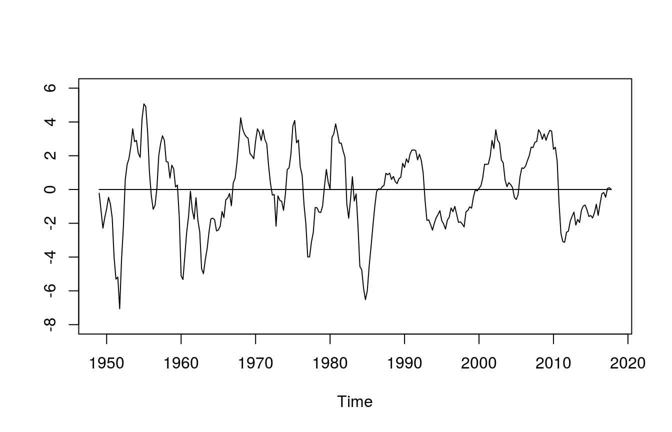
Plot annualised trend growth
temp <- apply(draws_tau, 2, diff) * 4
mean_dtau <- ts(apply(temp, 1, mean), start = 1949, frequency = 4)
plot(mean_dtau, plot.type = "single", ylim = c(1, 4.5), ylab = "")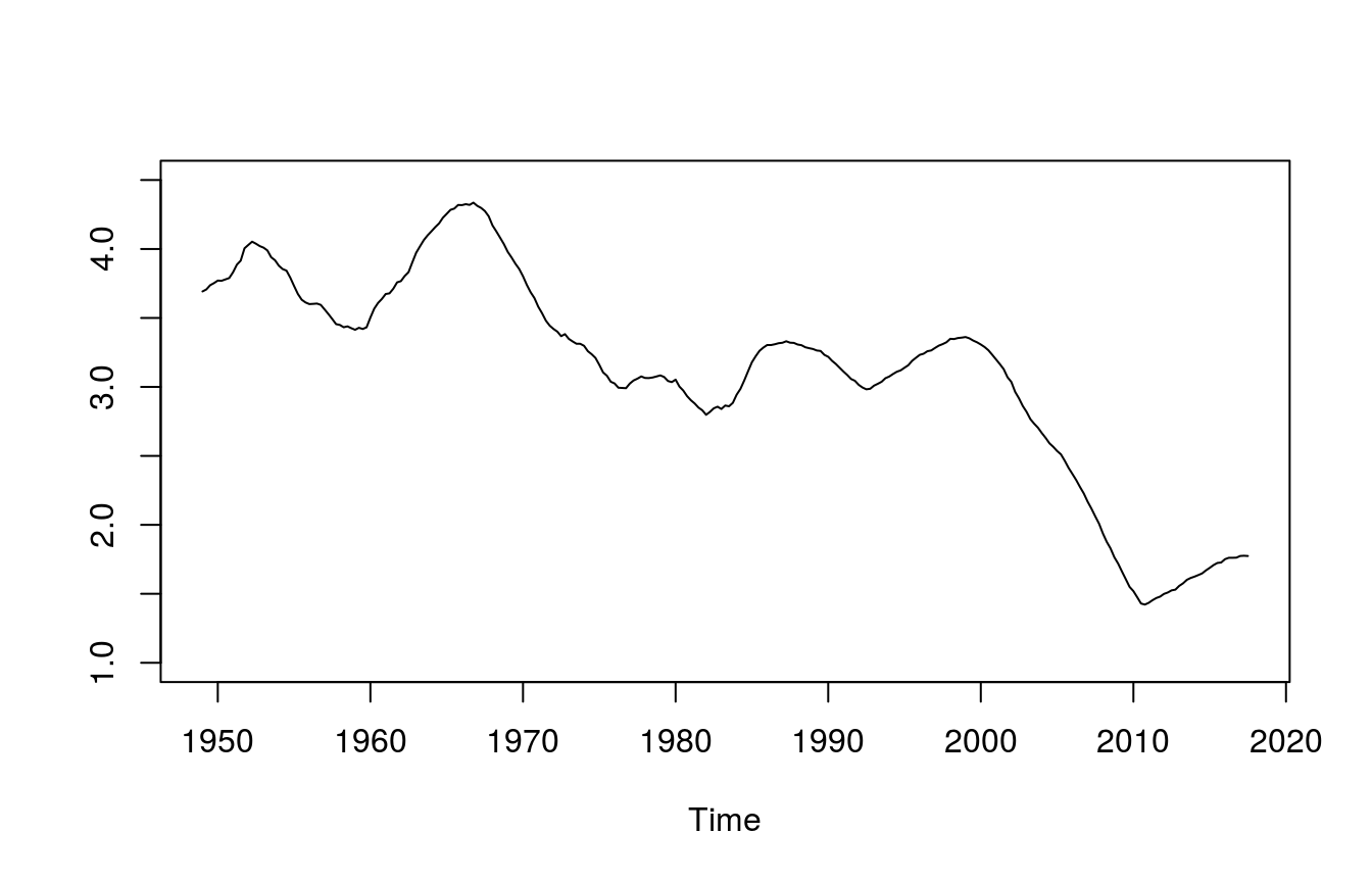
Work in progress