Chapter 8: Heteroskedasticity
library(wooldridge)Example 8.1
After loading the data and generating the dummy variables from chapter 7 estimate the model in the already familiar way.
data("wage1")

marrmale <- as.numeric(wage1$female == 0 & wage1$married == 1)
marrfem <- as.numeric(wage1$female == 1 & wage1$married == 1)
singfem <- as.numeric(wage1$female == 1 & wage1$married == 0)

lm.8.1 <- lm(lwage ~ marrmale + marrfem + singfem + educ + exper + expersq + tenure + tenursq, data = wage1)

summary(lm.8.1)
##
## Call:
## lm(formula = lwage ~ marrmale + marrfem + singfem + educ + exper +
## expersq + tenure + tenursq, data = wage1)
##
## Residuals:
## Min 1Q Median 3Q Max
## -1.89697 -0.24060 -0.02689 0.23144 1.09197
##
## Coefficients:
## Estimate Std. Error t value Pr(>|t|)
## (Intercept) 0.3213781 0.1000090 3.213 0.001393 **
## marrmale 0.2126757 0.0553572 3.842 0.000137 ***
## marrfem -0.1982676 0.0578355 -3.428 0.000656 ***
## singfem -0.1103502 0.0557421 -1.980 0.048272 *
## educ 0.0789103 0.0066945 11.787 < 2e-16 ***
## exper 0.0268006 0.0052428 5.112 4.50e-07 ***
## expersq -0.0005352 0.0001104 -4.847 1.66e-06 ***
## tenure 0.0290875 0.0067620 4.302 2.03e-05 ***
## tenursq -0.0005331 0.0002312 -2.306 0.021531 *
## ---
## Signif. codes: 0 '***' 0.001 '**' 0.01 '*' 0.05 '.' 0.1 ' ' 1
##
## Residual standard error: 0.3933 on 517 degrees of freedom
## Multiple R-squared: 0.4609, Adjusted R-squared: 0.4525
## F-statistic: 55.25 on 8 and 517 DF, p-value: < 2.2e-16The function coeftest from the lmtest package can be used to obtain the heteroskedasticity robust standard errors. The first argument of the function contains the result of the original estimation, i.e. lm.8.1.. The second argument tells R how to calculate the heteroskedasticity robust standard errors. Basically, you could just enter the first part and R would do the rest. However, since the standard procedure of coeftest would not give the same results as in the book, we have to specify them a bit. Thus, we use the vcovHC function from the sandwich package, which requires the output of the estimated model and a specification of the type of robust standard errors that should be calculated. In our case we want a simple White standard error, which is indicated by type = "HC0". Other, more sophisticated methods are described in the documentation of the function.
library("lmtest")## Loading required package: zoo##
## Attaching package: 'zoo'## The following objects are masked from 'package:base':
##
## as.Date, as.Date.numericlibrary("sandwich")
coeftest(lm.8.1, vcov=vcovHC(lm.8.1, type = "HC0"))##
## t test of coefficients:
##
## Estimate Std. Error t value Pr(>|t|)
## (Intercept) 0.32137808 0.10852843 2.9612 0.0032049 **
## marrmale 0.21267568 0.05665095 3.7541 0.0001937 ***
## marrfem -0.19826760 0.05826505 -3.4029 0.0007186 ***
## singfem -0.11035021 0.05662551 -1.9488 0.0518632 .
## educ 0.07891028 0.00735096 10.7347 < 2.2e-16 ***
## exper 0.02680057 0.00509497 5.2602 2.111e-07 ***
## expersq -0.00053525 0.00010543 -5.0770 5.360e-07 ***
## tenure 0.02908752 0.00688128 4.2270 2.800e-05 ***
## tenursq -0.00053314 0.00024159 -2.2068 0.0277670 *
## ---
## Signif. codes: 0 '***' 0.001 '**' 0.01 '*' 0.05 '.' 0.1 ' ' 1Example 8.2
data("gpa3")

lm.8.2 <- lm(cumgpa ~ sat + hsperc + tothrs + female + black + white,
             data = gpa3, subset = (term == 2))

summary(lm.8.2)
##
## Call:
## lm(formula = cumgpa ~ sat + hsperc + tothrs + female + black +
## white, data = gpa3, subset = (term == 2))
##
## Residuals:
## Min 1Q Median 3Q Max
## -1.54320 -0.29104 -0.02252 0.28348 1.24872
##
## Coefficients:
## Estimate Std. Error t value Pr(>|t|)
## (Intercept) 1.4700648 0.2298031 6.397 4.94e-10 ***
## sat 0.0011407 0.0001786 6.389 5.20e-10 ***
## hsperc -0.0085664 0.0012404 -6.906 2.27e-11 ***
## tothrs 0.0025040 0.0007310 3.426 0.000685 ***
## female 0.3034333 0.0590203 5.141 4.50e-07 ***
## black -0.1282837 0.1473701 -0.870 0.384616
## white -0.0587217 0.1409896 -0.416 0.677295
## ---
## Signif. codes: 0 '***' 0.001 '**' 0.01 '*' 0.05 '.' 0.1 ' ' 1
##
## Residual standard error: 0.4693 on 359 degrees of freedom
## Multiple R-squared: 0.4006, Adjusted R-squared: 0.3905
## F-statistic: 39.98 on 6 and 359 DF, p-value: < 2.2e-16coeftest(lm.8.2, vcov = vcovHC(lm.8.2, type = "HC0"))##
## t test of coefficients:
##
## Estimate Std. Error t value Pr(>|t|)
## (Intercept) 1.47006477 0.21855969 6.7261 6.888e-11 ***
## sat 0.00114073 0.00018969 6.0136 4.468e-09 ***
## hsperc -0.00856636 0.00140430 -6.1001 2.744e-09 ***
## tothrs 0.00250400 0.00073353 3.4136 0.0007142 ***
## female 0.30343329 0.05856959 5.1807 3.693e-07 ***
## black -0.12828368 0.11809549 -1.0863 0.2780880
## white -0.05872173 0.11032164 -0.5323 0.5948631
## ---
## Signif. codes: 0 '***' 0.001 '**' 0.01 '*' 0.05 '.' 0.1 ' ' 1For a heteroskedasticity robust F-test we perform a Wald-test. The procedure is similar to obtaining the coefficients’ standard errors. For the usual F-test estimate the restricted and unrestricted models and put their results into the anova function, which will print the F-statistic. For the Wald test we do the same, but this time we put the estimation results into the waldtest command and, as a third part of the function, you specify the method used to model heteroskedasticity.
lm.8.2.2 <- lm(cumgpa ~ sat + hsperc + tothrs + female, data = gpa3, subset = (term==2))

# Usual F-statistic
anova(lm.8.2, lm.8.2.2)
## Analysis of Variance Table
##
## Model 1: cumgpa ~ sat + hsperc + tothrs + female + black + white
## Model 2: cumgpa ~ sat + hsperc + tothrs + female
## Res.Df RSS Df Sum of Sq F Pr(>F)
## 1 359 79.062
## 2 361 79.362 -2 -0.29934 0.6796 0.5075Heteroskedasticity robust F-statistic
waldtest(lm.8.2, lm.8.2.2, vcov = vcovHC(lm.8.2, type = "HC0"))## Wald test
##
## Model 1: cumgpa ~ sat + hsperc + tothrs + female + black + white
## Model 2: cumgpa ~ sat + hsperc + tothrs + female
## Res.Df Df F Pr(>F)
## 1 359
## 2 361 -2 0.7478 0.4741Example 8.3
The first part of the example is similar to above. Estimate the model and print its summary and the heteroskedasticity robust standard errors.
# Load data and calculate the squared variable
data("crime1")

avgsensq <- crime1$avgsen^2

lm.8.3 <- lm(narr86 ~ pcnv + avgsen + avgsensq + ptime86 + qemp86 +
               inc86 + black + hispan, data = crime1)

summary(lm.8.3)
##
## Call:
## lm(formula = narr86 ~ pcnv + avgsen + avgsensq + ptime86 + qemp86 +
## inc86 + black + hispan, data = crime1)
##
## Residuals:
## Min 1Q Median 3Q Max
## -1.0008 -0.4515 -0.2391 0.2686 11.5307
##
## Coefficients:
## Estimate Std. Error t value Pr(>|t|)
## (Intercept) 0.5670128 0.0360573 15.725 < 2e-16 ***
## pcnv -0.1355954 0.0403699 -3.359 0.000794 ***
## avgsen 0.0178411 0.0096960 1.840 0.065872 .
## avgsensq -0.0005163 0.0002970 -1.738 0.082265 .
## ptime86 -0.0393600 0.0086935 -4.528 6.23e-06 ***
## qemp86 -0.0505072 0.0144345 -3.499 0.000474 ***
## inc86 -0.0014797 0.0003405 -4.345 1.44e-05 ***
## black 0.3246024 0.0454188 7.147 1.14e-12 ***
## hispan 0.1933800 0.0397035 4.871 1.18e-06 ***
## ---
## Signif. codes: 0 '***' 0.001 '**' 0.01 '*' 0.05 '.' 0.1 ' ' 1
##
## Residual standard error: 0.8284 on 2716 degrees of freedom
## Multiple R-squared: 0.0728, Adjusted R-squared: 0.07007
## F-statistic: 26.66 on 8 and 2716 DF, p-value: < 2.2e-16coeftest(lm.8.3, vcov = vcovHC(lm.8.3, type = "HC0"))##
## t test of coefficients:
##
## Estimate Std. Error t value Pr(>|t|)
## (Intercept) 0.56701278 0.04020901 14.1016 < 2.2e-16 ***
## pcnv -0.13559539 0.03356622 -4.0396 5.502e-05 ***
## avgsen 0.01784106 0.01010659 1.7653 0.0776275 .
## avgsensq -0.00051633 0.00020735 -2.4902 0.0128281 *
## ptime86 -0.03935998 0.00621327 -6.3348 2.772e-10 ***
## qemp86 -0.05050717 0.01417805 -3.5624 0.0003739 ***
## inc86 -0.00147966 0.00022913 -6.4576 1.256e-10 ***
## black 0.32460243 0.05841683 5.5567 3.017e-08 ***
## hispan 0.19338004 0.04023169 4.8067 1.618e-06 ***
## ---
## Signif. codes: 0 '***' 0.001 '**' 0.01 '*' 0.05 '.' 0.1 ' ' 1For the LM-test estimate the restricted model and regress its residuals on the variables of the unrestricted model. Obtain R-Squared and multiply it by the number of used observations to get the LM-value. Last, get the p-value.
lm.8.3.2 <- lm(narr86 ~ pcnv + ptime86 + qemp86 + inc86 +
                 black + hispan, data = crime1)

lm.8.3.2u <- lm(lm.8.3.2$residuals ~ pcnv + avgsen + avgsensq +
                  ptime86 + qemp86 + inc86 + black + hispan, data = crime1)

summary(lm.8.3.2u)$r.squared * 2725
## [1] 3.4626011 - pchisq(3.4626, 2)## [1] 0.1770541Example 8.4
For the Breusch-Pagan test estimate the model and obtain its squared residuals. Regress the latter on the variables of the model.
data("hprice1")

lm.e8.17 <- lm(price ~ lotsize + sqrft + bdrms, data = hprice1)
summary(lm.e8.17)
##
## Call:
## lm(formula = price ~ lotsize + sqrft + bdrms, data = hprice1)
##
## Residuals:
## Min 1Q Median 3Q Max
## -120.026 -38.530 -6.555 32.323 209.376
##
## Coefficients:
## Estimate Std. Error t value Pr(>|t|)
## (Intercept) -2.177e+01 2.948e+01 -0.739 0.46221
## lotsize 2.068e-03 6.421e-04 3.220 0.00182 **
## sqrft 1.228e-01 1.324e-02 9.275 1.66e-14 ***
## bdrms 1.385e+01 9.010e+00 1.537 0.12795
## ---
## Signif. codes: 0 '***' 0.001 '**' 0.01 '*' 0.05 '.' 0.1 ' ' 1
##
## Residual standard error: 59.83 on 84 degrees of freedom
## Multiple R-squared: 0.6724, Adjusted R-squared: 0.6607
## F-statistic: 57.46 on 3 and 84 DF, p-value: < 2.2e-16# Squared residuals
usq.17 <- (summary(lm.e8.17)$residual)^2
lm.e8.17u <- lm(usq.17 ~ lotsize + sqrft + bdrms, data = hprice1)
summary(lm.e8.17u)##
## Call:
## lm(formula = usq.17 ~ lotsize + sqrft + bdrms, data = hprice1)
##
## Residuals:
## Min 1Q Median 3Q Max
## -9044 -2212 -1256 -97 42582
##
## Coefficients:
## Estimate Std. Error t value Pr(>|t|)
## (Intercept) -5.523e+03 3.259e+03 -1.694 0.09390 .
## lotsize 2.015e-01 7.101e-02 2.838 0.00569 **
## sqrft 1.691e+00 1.464e+00 1.155 0.25128
## bdrms 1.042e+03 9.964e+02 1.046 0.29877
## ---
## Signif. codes: 0 '***' 0.001 '**' 0.01 '*' 0.05 '.' 0.1 ' ' 1
##
## Residual standard error: 6617 on 84 degrees of freedom
## Multiple R-squared: 0.1601, Adjusted R-squared: 0.1301
## F-statistic: 5.339 on 3 and 84 DF, p-value: 0.002048# LM-test
lm.e8.17u.2 <- lm(usq.17 ~ 1, data = hprice1)
lm.e8.17u.2u <- lm(summary(lm.e8.17u.2)$residuals ~ lotsize + sqrft + bdrms, data = hprice1)
summary(lm.e8.17u.2u)$r.squared * 88## [1] 14.092391 - pchisq(14.09239, 3)## [1] 0.002782054# Using logarithms
lm.e8.18 <- lm(lprice ~ llotsize + lsqrft + bdrms, data = hprice1)
summary(lm.e8.18)##
## Call:
## lm(formula = lprice ~ llotsize + lsqrft + bdrms, data = hprice1)
##
## Residuals:
## Min 1Q Median 3Q Max
## -0.68422 -0.09178 -0.01584 0.11213 0.66899
##
## Coefficients:
## Estimate Std. Error t value Pr(>|t|)
## (Intercept) -1.29704 0.65128 -1.992 0.0497 *
## llotsize 0.16797 0.03828 4.388 3.31e-05 ***
## lsqrft 0.70023 0.09287 7.540 5.01e-11 ***
## bdrms 0.03696 0.02753 1.342 0.1831
## ---
## Signif. codes: 0 '***' 0.001 '**' 0.01 '*' 0.05 '.' 0.1 ' ' 1
##
## Residual standard error: 0.1846 on 84 degrees of freedom
## Multiple R-squared: 0.643, Adjusted R-squared: 0.6302
## F-statistic: 50.42 on 3 and 84 DF, p-value: < 2.2e-16# Breusch-Pagan test
usq.18 <- (summary(lm.e8.18)$residual)^2
lm.e8.18u <- lm(usq.18 ~ llotsize + lsqrft + bdrms, data = hprice1)
summary(lm.e8.18u)##
## Call:
## lm(formula = usq.18 ~ llotsize + lsqrft + bdrms, data = hprice1)
##
## Residuals:
## Min 1Q Median 3Q Max
## -0.05601 -0.03011 -0.01687 0.00523 0.40978
##
## Coefficients:
## Estimate Std. Error t value Pr(>|t|)
## (Intercept) 0.509994 0.257857 1.978 0.0512 .
## llotsize -0.007016 0.015156 -0.463 0.6446
## lsqrft -0.062737 0.036767 -1.706 0.0916 .
## bdrms 0.016841 0.010900 1.545 0.1261
## ---
## Signif. codes: 0 '***' 0.001 '**' 0.01 '*' 0.05 '.' 0.1 ' ' 1
##
## Residual standard error: 0.07309 on 84 degrees of freedom
## Multiple R-squared: 0.04799, Adjusted R-squared: 0.01399
## F-statistic: 1.412 on 3 and 84 DF, p-value: 0.2451# LM-test
summary(lm.e8.18u)$r.squared * 88## [1] 4.2232481 - pchisq(4.223248, 3)## [1] 0.2383446Example 8.5
To obtain the test statistic of the the White test, estimate the model, obtain its squared residuals, fitted values and squared fitted values and regress the first on the latter ones. Then, get the R-Squared and multiply it by the number of used observations to get the LM-statistic and the p-value.
data("hprice1")

lm.e8.18 <- lm(lprice ~ llotsize + lsqrft + bdrms, data = hprice1)
ressq <- lm.e8.18$residuals^2
fitted <- lm.e8.18$fitted.values
fittedsq <- lm.e8.18$fitted.values^2
rsq <- summary(lm(ressq ~ fitted + fittedsq))$r.squared

rsq * 88
## [1] 3.4472861 - pchisq(3.447286, 2)## [1] 0.178415Example 8.6
For weighted least squares you can still use R’s lm command, but you have to tell R how to weigh the observations with respect to the variance of the coefficients. This is achieved by specifying the argument weights as 1/h, where in our example h is income. Now the model can be estimated and since we have controlled for heteroskedasticity by specifying weights, we can use the usual summary command to get heteroskedasticity robust results and do not need to use coeftest.
data("k401ksubs")

lm.8.6.1 <- lm(nettfa ~ inc, data = k401ksubs, subset = (fsize == 1))
coeftest(lm.8.6.1, vcov = vcovHC(lm.8.6.1, type = "HC0"))
##
## t test of coefficients:
##
## Estimate Std. Error t value Pr(>|t|)
## (Intercept) -10.57095 2.52902 -4.1799 3.042e-05 ***
## inc 0.82068 0.10354 7.9261 3.711e-15 ***
## ---
## Signif. codes: 0 '***' 0.001 '**' 0.01 '*' 0.05 '.' 0.1 ' ' 1lm.8.6.2 <- lm(nettfa ~ inc, weights = 1/inc, data = k401ksubs, subset = (fsize == 1))
summary(lm.8.6.2)##
## Call:
## lm(formula = nettfa ~ inc, data = k401ksubs, subset = (fsize ==
## 1), weights = 1/inc)
##
## Weighted Residuals:
## Min 1Q Median 3Q Max
## -23.469 -2.339 -1.086 0.352 178.220
##
## Coefficients:
## Estimate Std. Error t value Pr(>|t|)
## (Intercept) -9.58070 1.65328 -5.795 7.91e-09 ***
## inc 0.78705 0.06348 12.398 < 2e-16 ***
## ---
## Signif. codes: 0 '***' 0.001 '**' 0.01 '*' 0.05 '.' 0.1 ' ' 1
##
## Residual standard error: 7.219 on 2015 degrees of freedom
## Multiple R-squared: 0.07088, Adjusted R-squared: 0.07042
## F-statistic: 153.7 on 1 and 2015 DF, p-value: < 2.2e-16age.25sq <- (k401ksubs$age - 25)^2
lm.8.6.3 <- lm(nettfa ~ age.25sq + male + e401k,
data = k401ksubs, subset = (fsize == 1))
coeftest(lm.8.6.3, vcov = vcovHC(lm.8.6.3, type = "HC0"))##
## t test of coefficients:
##
## Estimate Std. Error t value Pr(>|t|)
## (Intercept) -2.3360343 1.8725857 -1.2475 0.21236
## age.25sq 0.0258052 0.0044892 5.7483 1.039e-08 ***
## male 5.3883568 2.2771296 2.3663 0.01806 *
## e401k 13.1199818 2.4341139 5.3900 7.870e-08 ***
## ---
## Signif. codes: 0 '***' 0.001 '**' 0.01 '*' 0.05 '.' 0.1 ' ' 1lm.8.6.4 <- lm(nettfa ~ inc + age.25sq + male + e401k, weights = 1 / inc,
data = k401ksubs, subset = (fsize == 1))
summary(lm.8.6.4)##
## Call:
## lm(formula = nettfa ~ inc + age.25sq + male + e401k, data = k401ksubs,
## subset = (fsize == 1), weights = 1/inc)
##
## Weighted Residuals:
## Min 1Q Median 3Q Max
## -26.613 -2.491 -0.803 0.934 178.052
##
## Coefficients:
## Estimate Std. Error t value Pr(>|t|)
## (Intercept) -16.702521 1.957995 -8.530 < 2e-16 ***
## inc 0.740384 0.064303 11.514 < 2e-16 ***
## age.25sq 0.017537 0.001931 9.080 < 2e-16 ***
## male 1.840529 1.563587 1.177 0.23929
## e401k 5.188281 1.703426 3.046 0.00235 **
## ---
## Signif. codes: 0 '***' 0.001 '**' 0.01 '*' 0.05 '.' 0.1 ' ' 1
##
## Residual standard error: 7.065 on 2012 degrees of freedom
## Multiple R-squared: 0.1115, Adjusted R-squared: 0.1097
## F-statistic: 63.13 on 4 and 2012 DF, p-value: < 2.2e-16Example 8.7
data("smoke")

lm.8.7 <- lm(cigs ~ lincome + lcigpric + educ + age + agesq + restaurn, data = smoke)
summary(lm.8.7)
##
## Call:
## lm(formula = cigs ~ lincome + lcigpric + educ + age + agesq +
## restaurn, data = smoke)
##
## Residuals:
## Min 1Q Median 3Q Max
## -15.819 -9.381 -5.975 7.922 70.221
##
## Coefficients:
## Estimate Std. Error t value Pr(>|t|)
## (Intercept) -3.639841 24.078660 -0.151 0.87988
## lincome 0.880268 0.727783 1.210 0.22682
## lcigpric -0.750859 5.773343 -0.130 0.89655
## educ -0.501498 0.167077 -3.002 0.00277 **
## age 0.770694 0.160122 4.813 1.78e-06 ***
## agesq -0.009023 0.001743 -5.176 2.86e-07 ***
## restaurn -2.825085 1.111794 -2.541 0.01124 *
## ---
## Signif. codes: 0 '***' 0.001 '**' 0.01 '*' 0.05 '.' 0.1 ' ' 1
##
## Residual standard error: 13.4 on 800 degrees of freedom
## Multiple R-squared: 0.05274, Adjusted R-squared: 0.04563
## F-statistic: 7.423 on 6 and 800 DF, p-value: 9.499e-08# Breusch-Pagan
summary(lm.8.7u <-lm(lm.8.7$residuals^2 ~ lincome + lcigpric +
educ + age + agesq + restaurn, data = smoke))##
## Call:
## lm(formula = lm.8.7$residuals^2 ~ lincome + lcigpric + educ +
## age + agesq + restaurn, data = smoke)
##
## Residuals:
## Min 1Q Median 3Q Max
## -270.1 -127.5 -94.0 -39.1 4667.8
##
## Coefficients:
## Estimate Std. Error t value Pr(>|t|)
## (Intercept) -636.30306 652.49456 -0.975 0.3298
## lincome 24.63848 19.72180 1.249 0.2119
## lcigpric 60.97655 156.44869 0.390 0.6968
## educ -2.38423 4.52753 -0.527 0.5986
## age 19.41748 4.33907 4.475 8.75e-06 ***
## agesq -0.21479 0.04723 -4.547 6.27e-06 ***
## restaurn -71.18138 30.12789 -2.363 0.0184 *
## ---
## Signif. codes: 0 '***' 0.001 '**' 0.01 '*' 0.05 '.' 0.1 ' ' 1
##
## Residual standard error: 363.2 on 800 degrees of freedom
## Multiple R-squared: 0.03997, Adjusted R-squared: 0.03277
## F-statistic: 5.552 on 6 and 800 DF, p-value: 1.189e-05summary(lm.8.7u)$r.squared * 807## [1] 32.258421 - pchisq(summary(lm.8.7u)$r.squared*807, 6)## [1] 1.455779e-05For feasible GLS you obtain the logarithm of squared residuals from the basic model. Then you regress it on the model’s independent variables and calculate the exponential of fitted values from that regression which gives hhat. Then you estimate the basic model again, but with the weights 1/hhat.
lres.u <- log(lm.8.7$residuals^2)
lm.8.7gls.u <- lm(lres.u ~ lincome + lcigpric + educ + age +
                    agesq + restaurn, data = smoke)
hhat <- exp(lm.8.7gls.u$fitted.values)
lm.8.7gls <- lm(cigs ~ lincome + lcigpric + educ + age +
agesq + restaurn, weights = 1 / hhat, data = smoke)
summary(lm.8.7gls)##
## Call:
## lm(formula = cigs ~ lincome + lcigpric + educ + age + agesq +
## restaurn, data = smoke, weights = 1/hhat)
##
## Weighted Residuals:
## Min 1Q Median 3Q Max
## -1.9036 -0.9532 -0.8099 0.8415 9.8556
##
## Coefficients:
## Estimate Std. Error t value Pr(>|t|)
## (Intercept) 5.6354618 17.8031385 0.317 0.751673
## lincome 1.2952399 0.4370118 2.964 0.003128 **
## lcigpric -2.9403123 4.4601445 -0.659 0.509930
## educ -0.4634464 0.1201587 -3.857 0.000124 ***
## age 0.4819479 0.0968082 4.978 7.86e-07 ***
## agesq -0.0056272 0.0009395 -5.990 3.17e-09 ***
## restaurn -3.4610641 0.7955050 -4.351 1.53e-05 ***
## ---
## Signif. codes: 0 '***' 0.001 '**' 0.01 '*' 0.05 '.' 0.1 ' ' 1
##
## Residual standard error: 1.579 on 800 degrees of freedom
## Multiple R-squared: 0.1134, Adjusted R-squared: 0.1068
## F-statistic: 17.06 on 6 and 800 DF, p-value: < 2.2e-16Table 8.2
# Recall the first column of the table
summary(lm.8.6.4)
##
## Call:
## lm(formula = nettfa ~ inc + age.25sq + male + e401k, data = k401ksubs,
## subset = (fsize == 1), weights = 1/inc)
##
## Weighted Residuals:
## Min 1Q Median 3Q Max
## -26.613 -2.491 -0.803 0.934 178.052
##
## Coefficients:
## Estimate Std. Error t value Pr(>|t|)
## (Intercept) -16.702521 1.957995 -8.530 < 2e-16 ***
## inc 0.740384 0.064303 11.514 < 2e-16 ***
## age.25sq 0.017537 0.001931 9.080 < 2e-16 ***
## male 1.840529 1.563587 1.177 0.23929
## e401k 5.188281 1.703426 3.046 0.00235 **
## ---
## Signif. codes: 0 '***' 0.001 '**' 0.01 '*' 0.05 '.' 0.1 ' ' 1
##
## Residual standard error: 7.065 on 2012 degrees of freedom
## Multiple R-squared: 0.1115, Adjusted R-squared: 0.1097
## F-statistic: 63.13 on 4 and 2012 DF, p-value: < 2.2e-16# Column 2
coeftest(lm.8.6.4, vcov = vcovHC(lm.8.6.4, type = "HC0"))##
## t test of coefficients:
##
## Estimate Std. Error t value Pr(>|t|)
## (Intercept) -16.7025205 2.2402025 -7.4558 1.320e-13 ***
## inc 0.7403843 0.0749626 9.8767 < 2.2e-16 ***
## age.25sq 0.0175373 0.0025817 6.7930 1.442e-11 ***
## male 1.8405293 1.3091836 1.4059 0.159920
## e401k 5.1882807 1.5699057 3.3048 0.000967 ***
## ---
## Signif. codes: 0 '***' 0.001 '**' 0.01 '*' 0.05 '.' 0.1 ' ' 1Example 8.8
With respect to linear probability models the procedure is rather similar to the first examples: estimate the model and use coeftest to get heteroskedasticity robust estimates of the standard errors.
data("mroz")

lm.8.8 <- lm(inlf ~ nwifeinc + educ + exper + expersq +
               age + kidslt6 + kidsge6, data = mroz)

summary(lm.8.8)
##
## Call:
## lm(formula = inlf ~ nwifeinc + educ + exper + expersq + age +
## kidslt6 + kidsge6, data = mroz)
##
## Residuals:
## Min 1Q Median 3Q Max
## -0.93432 -0.37526 0.08833 0.34404 0.99417
##
## Coefficients:
## Estimate Std. Error t value Pr(>|t|)
## (Intercept) 0.5855192 0.1541780 3.798 0.000158 ***
## nwifeinc -0.0034052 0.0014485 -2.351 0.018991 *
## educ 0.0379953 0.0073760 5.151 3.32e-07 ***
## exper 0.0394924 0.0056727 6.962 7.38e-12 ***
## expersq -0.0005963 0.0001848 -3.227 0.001306 **
## age -0.0160908 0.0024847 -6.476 1.71e-10 ***
## kidslt6 -0.2618105 0.0335058 -7.814 1.89e-14 ***
## kidsge6 0.0130122 0.0131960 0.986 0.324415
## ---
## Signif. codes: 0 '***' 0.001 '**' 0.01 '*' 0.05 '.' 0.1 ' ' 1
##
## Residual standard error: 0.4271 on 745 degrees of freedom
## Multiple R-squared: 0.2642, Adjusted R-squared: 0.2573
## F-statistic: 38.22 on 7 and 745 DF, p-value: < 2.2e-16coeftest(lm.8.8, vcov = vcovHC(lm.8.8, type = "HC0"))##
## t test of coefficients:
##
## Estimate Std. Error t value Pr(>|t|)
## (Intercept) 0.58551922 0.15144889 3.8661 0.0001202 ***
## nwifeinc -0.00340517 0.00151681 -2.2450 0.0250635 *
## educ 0.03799530 0.00722734 5.2572 1.913e-07 ***
## exper 0.03949239 0.00577907 6.8337 1.722e-11 ***
## expersq -0.00059631 0.00018899 -3.1552 0.0016683 **
## age -0.01609081 0.00238623 -6.7432 3.108e-11 ***
## kidslt6 -0.26181047 0.03161391 -8.2815 5.626e-16 ***
## kidsge6 0.01301223 0.01346085 0.9667 0.3340215
## ---
## Signif. codes: 0 '***' 0.001 '**' 0.01 '*' 0.05 '.' 0.1 ' ' 1Example 8.9
Since linear probability models automatically suffer from heteroskedasticity, we have to somehow control for that. The first part of the estimation is already familiar.
data("gpa1")

# Generate dummy variable vector which is 1 when either the
# father or the mother or both were at college.
parcoll <- as.numeric(gpa1$fathcoll == 1 | gpa1$mothcoll)

lm.8.9 <- lm(PC ~ hsGPA + ACT + parcoll, data = gpa1)

summary(lm.8.9)
##
## Call:
## lm(formula = PC ~ hsGPA + ACT + parcoll, data = gpa1)
##
## Residuals:
## Min 1Q Median 3Q Max
## -0.4915 -0.4494 -0.2437 0.5375 0.8223
##
## Coefficients:
## Estimate Std. Error t value Pr(>|t|)
## (Intercept) -0.0004322 0.4905358 -0.001 0.9993
## hsGPA 0.0653943 0.1372576 0.476 0.6345
## ACT 0.0005645 0.0154967 0.036 0.9710
## parcoll 0.2210541 0.0929570 2.378 0.0188 *
## ---
## Signif. codes: 0 '***' 0.001 '**' 0.01 '*' 0.05 '.' 0.1 ' ' 1
##
## Residual standard error: 0.486 on 137 degrees of freedom
## Multiple R-squared: 0.04153, Adjusted R-squared: 0.02054
## F-statistic: 1.979 on 3 and 137 DF, p-value: 0.1201coeftest(lm.8.9, vcov = vcovHC(lm.8.9, type = "HC0"))##
## t test of coefficients:
##
## Estimate Std. Error t value Pr(>|t|)
## (Intercept) -0.00043220 0.48879587 -0.0009 0.99930
## hsGPA 0.06539435 0.13946545 0.4689 0.63989
## ACT 0.00056451 0.01584133 0.0356 0.97163
## parcoll 0.22105405 0.08678002 2.5473 0.01196 *
## ---
## Signif. codes: 0 '***' 0.001 '**' 0.01 '*' 0.05 '.' 0.1 ' ' 1To deal with heteroskedasticity obtain the fitted values from the basic model and check whether all of them are neither negative nor above unity. I plotted a histogram for that. You might also lock at min and max or functions like that. Then calculate hhat as described in the book and use its inverse (1/hhat) for the weights specification in the final regression.
hist(lm.8.9$fitted.values) # Fitted values are neither negative nor above unity.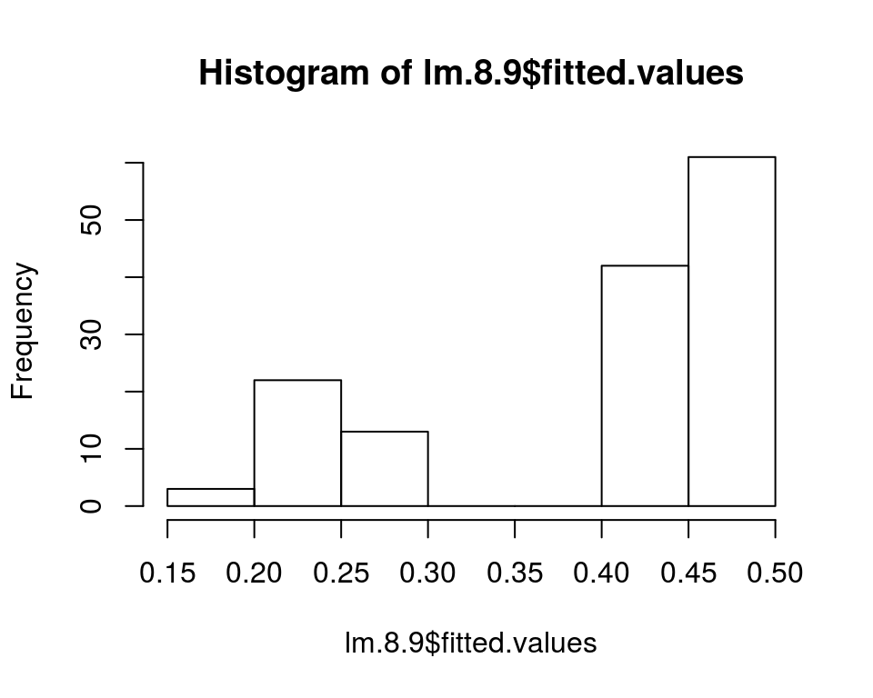
hhat <- lm.8.9$fitted.values * (1 - lm.8.9$fitted.values) # Calculate hhat (h = yhat * (1 - yhat))
lm.8.9wls <- lm(PC ~ hsGPA + ACT + parcoll, weights = 1 / hhat, data = gpa1)
summary(lm.8.9wls)
##
## Call:
## lm(formula = PC ~ hsGPA + ACT + parcoll, data = gpa1, weights = 1/hhat)
##
## Weighted Residuals:
## Min 1Q Median 3Q Max
## -1.0015 -0.9029 -0.5576 1.0800 2.0429
##
## Coefficients:
## Estimate Std. Error t value Pr(>|t|)
## (Intercept) 0.026210 0.476650 0.055 0.9562
## hsGPA 0.032703 0.129882 0.252 0.8016
## ACT 0.004272 0.015453 0.276 0.7826
## parcoll 0.215186 0.086292 2.494 0.0138 *
## ---
## Signif. codes: 0 '***' 0.001 '**' 0.01 '*' 0.05 '.' 0.1 ' ' 1
##
## Residual standard error: 1.016 on 137 degrees of freedom
## Multiple R-squared: 0.04644, Adjusted R-squared: 0.02556
## F-statistic: 2.224 on 3 and 137 DF, p-value: 0.08816For a further very interesting article on dealing with heteroskedasticity in R I recommend this page.