Bayesian Inference of Structural Vector Autoregressions (SVAR) with the `bvartools` package
Posted in r var with tags r var svar vector autoregression bvartools -The bvartools allows to perform Bayesian inference of Vector autoregressive (VAR) models, including structural VARs. This post guides through the Bayesian inference of SVAR models in R using the bvartools package.
Data
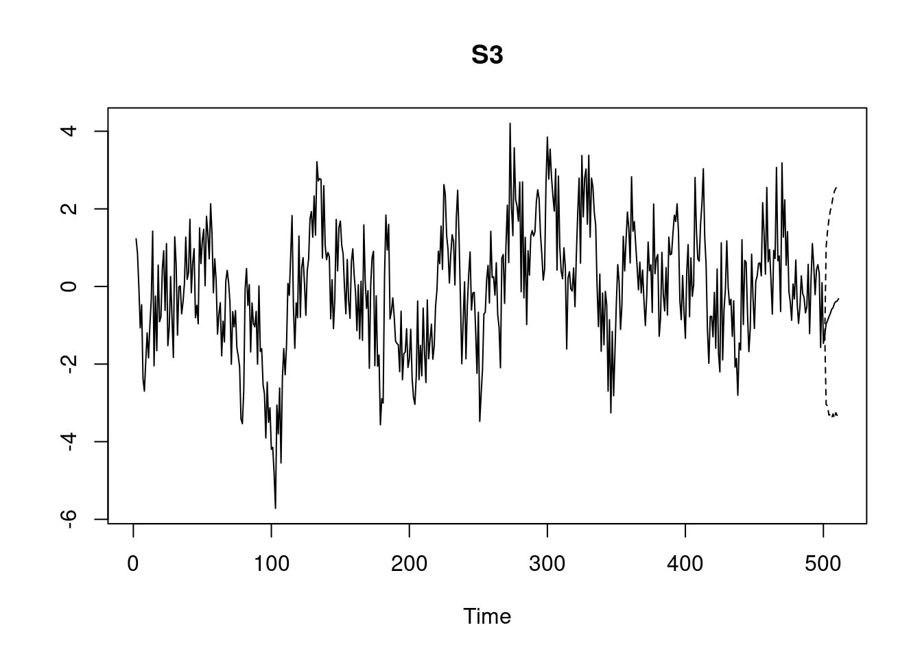
For this illustration we generate an artificial data set with three endogenous variables, which follows the data generating process
\[y_t = A_1 y_{t - 1} + B \epsilon_t,\]
where
\[ A_1 = \begin{bmatrix} 0.3 & 0.12 & 0.69 \\ 0 & 0.3 & 0.48 \\ 0.24 & 0.24 & 0.3 \end{bmatrix} \text{, } B = \begin{bmatrix} 1 & 0 & 0 \\ -0.14 & 1 & 0 \\ -0.06 & 0.39 & 1 \end{bmatrix} \text{ and } \epsilon_t \sim N(0, I_3). \]
# Reset random number generator for reproducibility
set.seed(24579)

tt <- 500 # Number of time series observations

# Coefficient matrix
A_1 <- matrix(c(0.3, 0, 0.24,
                0.12, 0.3, 0.24,
                0.69, 0.48, 0.3), 3)

# Structural coefficients
B <- diag(1, 3)
B[lower.tri(B)] <- c(-0.14, -0.06, 0.39)

# Generate series
sd_sigma <- 1
series <- matrix(rnorm(3, 0, sd_sigma), 3, tt + 1) # Raw series with zeros
for (i in 2:(tt + 1)){
  series[, i] <- A_1 %*% series[, i - 1] +  B %*% rnorm(3, 0, sd_sigma)
}

series <- ts(t(series)) # Convert to time series object
dimnames(series)[[2]] <- c("S1", "S2", "S3") # Rename variables

# Plot the series
plot.ts(series, main = "Artificial time series")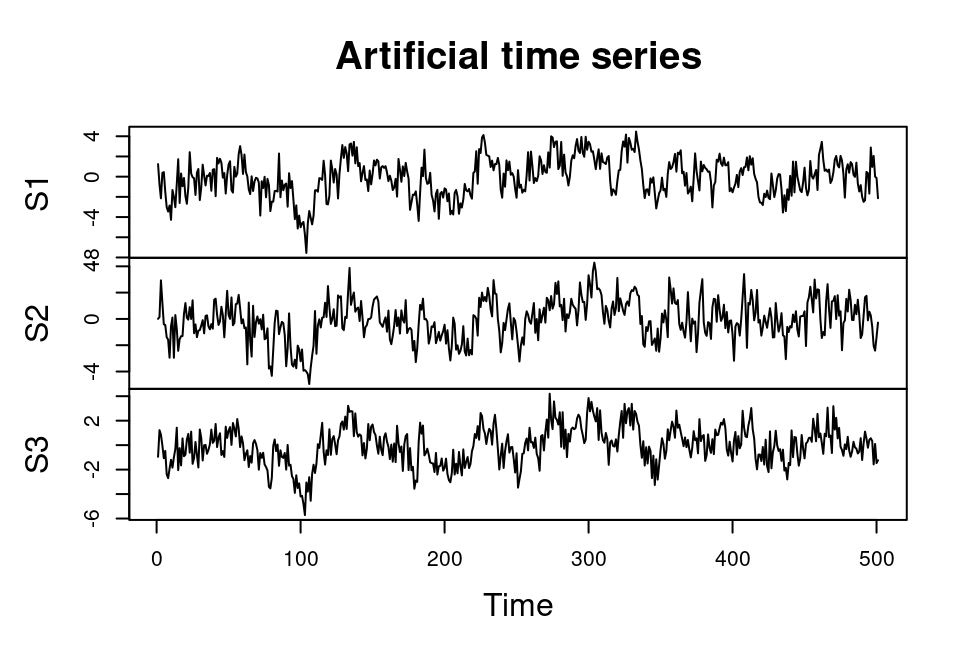
Model generation
library(bvartools)

# Generate basic model
mod <- gen_var(series,
               p = 1,
               deterministic = "none",
               structural = TRUE,
               iterations = 5000,
               burnin = 2000)
Prior specification
mod_w_prior <- add_priors(mod,
                          coef = list(v_i = 0),
                          sigma = list(shape = 3, rate = .0001))
Draw posteriors
post <- draw_posterior(mod_w_prior)Evaluation
Summary statistics
summary(post)##
## Bayesian SVAR model with p = 1
##
## Model:
##
## y ~ S1.01 + S2.01 + S3.01 + S1 + S2 + S3
##
## Variable: S1
##
## Mean SD Naive SD Time-series SD 2.5% 50% 97.5%
## S1.01 0.3293 0.02966 0.0004195 0.0004195 0.27280 0.3294 0.3884
## S2.01 0.1118 0.04009 0.0005670 0.0005670 0.03324 0.1115 0.1908
## S3.01 0.6810 0.04188 0.0005923 0.0005923 0.59815 0.6812 0.7624
## S1 1.0000 0.00000 0.0000000 0.0000000 1.00000 1.0000 1.0000
## S2 0.0000 0.00000 0.0000000 0.0000000 0.00000 0.0000 0.0000
## S3 0.0000 0.00000 0.0000000 0.0000000 0.00000 0.0000 0.0000
##
## Variable: S2
##
## Mean SD Naive SD Time-series SD 2.5% 50% 97.5%
## S1.01 0.05776 0.03355 0.0004745 0.0004745 -0.006956 0.05779 0.1239
## S2.01 0.30951 0.04081 0.0005771 0.0005771 0.230628 0.30994 0.3895
## S3.01 0.63676 0.05263 0.0007443 0.0007443 0.537193 0.63656 0.7400
## S1 0.18192 0.04636 0.0006556 0.0006556 0.092993 0.18148 0.2728
## S2 1.00000 0.00000 0.0000000 0.0000000 1.000000 1.00000 1.0000
## S3 0.00000 0.00000 0.0000000 0.0000000 0.000000 0.00000 0.0000
##
## Variable: S3
##
## Mean SD Naive SD Time-series SD 2.5% 50% 97.5%
## S1.01 0.25778 0.03293 0.0004657 0.0004657 0.19234 0.25788 0.3200
## S2.01 0.16723 0.04260 0.0006024 0.0006024 0.08265 0.16773 0.2490
## S3.01 0.19244 0.05762 0.0008148 0.0008148 0.07971 0.19282 0.3057
## S1 0.05055 0.04507 0.0006374 0.0005991 -0.03931 0.05031 0.1371
## S2 -0.31257 0.04345 0.0006145 0.0006145 -0.39792 -0.31234 -0.2277
## S3 1.00000 0.00000 0.0000000 0.0000000 1.00000 1.00000 1.0000
##
## Variance-covariance matrix:
##
## Mean SD Naive SD Time-series SD 2.5% 50% 97.5%
## S1_S1 0.9880 0.06301 0.0008911 0.0009084 0.8745 0.9836 1.125
## S1_S2 0.0000 0.00000 0.0000000 0.0000000 0.0000 0.0000 0.000
## S1_S3 0.0000 0.00000 0.0000000 0.0000000 0.0000 0.0000 0.000
## S2_S1 0.0000 0.00000 0.0000000 0.0000000 0.0000 0.0000 0.000
## S2_S2 1.0375 0.06675 0.0009440 0.0009440 0.9135 1.0349 1.174
## S2_S3 0.0000 0.00000 0.0000000 0.0000000 0.0000 0.0000 0.000
## S3_S1 0.0000 0.00000 0.0000000 0.0000000 0.0000 0.0000 0.000
## S3_S2 0.0000 0.00000 0.0000000 0.0000000 0.0000 0.0000 0.000
## S3_S3 0.9862 0.06326 0.0008947 0.0009085 0.8692 0.9831 1.120Compare with actual values
solve(B) %*% A_1## [,1] [,2] [,3]
## [1,] 0.30000 0.120000 0.690000
## [2,] 0.04200 0.316800 0.576600
## [3,] 0.24162 0.123648 0.116526solve(B)## [,1] [,2] [,3]
## [1,] 1.0000 0.00 0
## [2,] 0.1400 1.00 0
## [3,] 0.0054 -0.39 1Plotting posterior distributions
t
plot(post, type = "boxplot")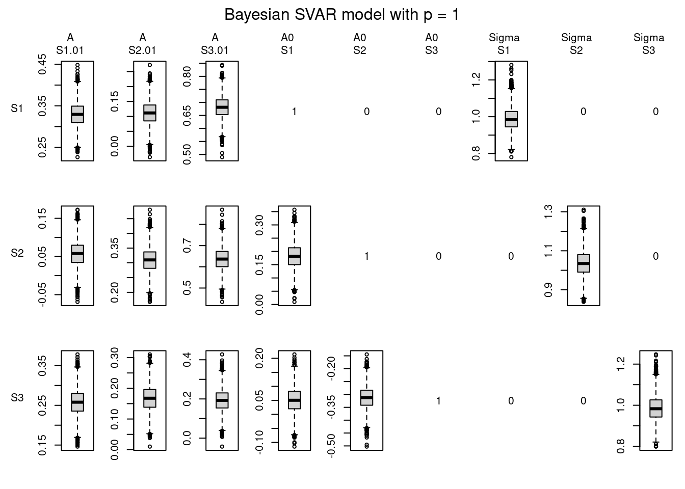
Forecasts
pred_svar <- predict(post, "S1", n.ahead = 10)

plot(pred_svar)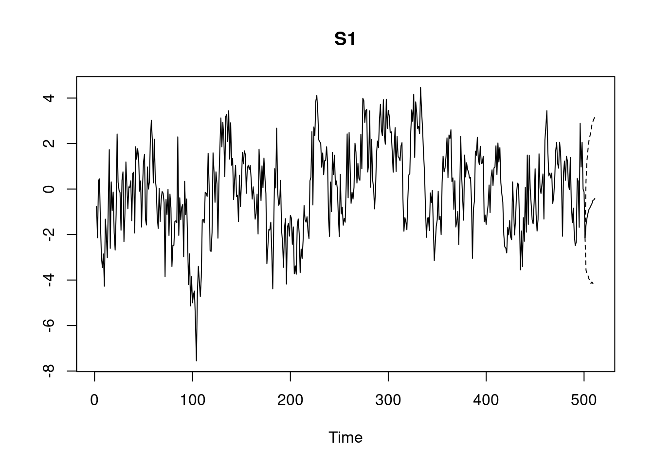
Impulse response functions
irf_svar <- irf(post, n.ahead = 10, impulse = "S1", response = "S3", type = "sir")

plot(irf_svar)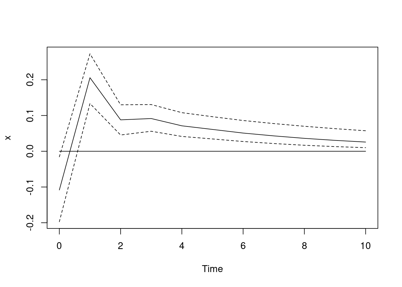
Variance decomposition
fevd_svar <- fevd(post, n.ahead = 10, response = "S3", type = "sir")

plot(fevd_svar)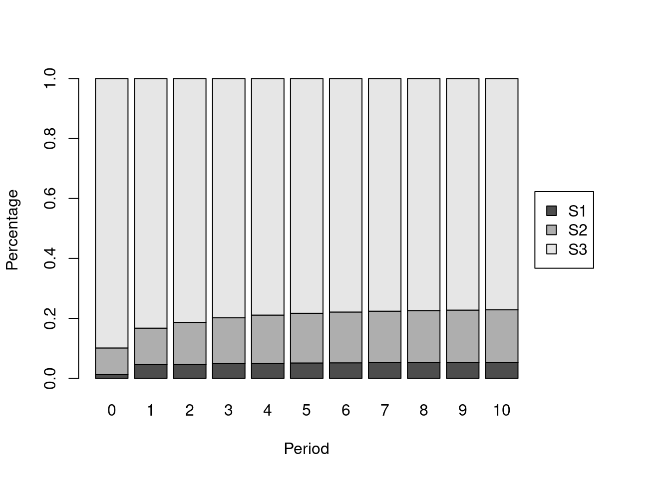
Compare with frequentist results
Estimate basic VAR
library(vars)

freq_var <- VAR(series, p = 1, type = "none")
Estimate structural coefficients
# Specify A0
a <- diag(1, 3)
a[lower.tri(a)] <- NA

freq_var_a <- SVAR(freq_var, Amat = a, max.iter = 1000)

freq_var_a
##
## SVAR Estimation Results:
## ========================
##
##
## Estimated A matrix:
## S1 S2 S3
## S1 1.00000 0.0000 0
## S2 0.18177 1.0000 0
## S3 0.05078 -0.3132 1Impulse response function
freq_var_irf <- irf(freq_var_a, n.ahead = 10, impulse = "S1", response = "S3")

plot(freq_var_irf)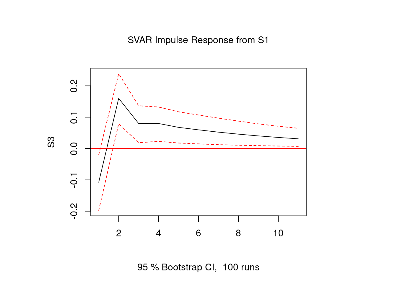
Literature
Chan, J., Koop, G., Poirier, D. J., & Tobias, J. L. (2019). Bayesian Econometric Methods (2nd ed.). Cambridge: University Press.
Lütkepohl, H. (2007). New Introduction to Multiple Time Series Analyis (2nd ed.). Berlin: Springer.
Pfaff, B. (2008). VAR, SVAR and SVEC models: Implementation within R package vars. Journal of Statistical Software, 27(4).