An Introduction to Bayesian VAR (BVAR) Models
with tags r bvar var bayes bayesian-var bvartools gibbs-sampler -BVAR models
Bayesian VAR (BVAR) models have the same mathematical form as any other VAR model, i.e.
\[ y_t = c + \sum_{l=i}^{p} A_i y_{t-i} + \epsilon_t,\] where \(y_t\) is a \(K \times 1\) vector of endogenous variables in period \(t\), \(A_i\) is the cofficient matrix corresponding to the \(i\)th lag of \(y_t\), \(c\) is a constant deterministic term and \(\epsilon\) is an error term with zero mean and variance-covariance \(\Sigma\).
The only difference between usual VAR models and BVAR models is the way parameter estimates are obtained and interpreted. VAR models are usually estimated by OLS, which is a simple and computationally fast estimator. By contrast, Bayesian estimators are slightly more complicated and more burdensome in terms of algebra and calculation power. The coefficients obtained by so-called frequentist estimators like OLS are interpreted based on the concept of the sampling distribution. In Bayesian inference, the coefficients are assumed to have their own distribution. A more detailed treatment of the difference between frequentist and Bayesian inference can be found in Kennedy (2008, ch. 14), which provides a short introduction to the Bayesian approach and a series of references for interested readers. Koop and Korobilis (2010) provide a very good introduction to Bayesian VAR estimators.
As already mentioned, Bayesian inference can be algebraically demanding. However, Bayesian estimators for linear VAR models can be implemented in a straightforward manner. A standard implementation is a so-called Gibbs sampler, which belongs to the family of Markov-Chain-Monte-Carlo (MCMC) methods. A detailed treatment of this method is beyond the scope of this post, but Wikipedia might be a good start to become familiar with it. Personally, I like to think of the Gibbs sampler as throwing a bunch of random numbers at a model and see what sticks. The remainer of this text provides the code to set up and estimate a basic BVAR model with the bvartools package.
Model and data
For this illustration the dataset E1 from Lütkepohl (2007) is used. It contains data on West German fixed investment, disposable income and consumption expenditures in billions of DM from 1960Q1 to 1982Q4. Following Lütkepohl (2007) the VAR model has two lags, i.e. \(p = 2\) and only the first 73 observations are used for inference.
library(bvartools)

data("e1") # Load the data
e1 <- diff(log(e1)) # Calculate first-log-differences

# Reduce number of oberservations
e1 <- window(e1, end = c(1978, 4))
Basically, it would be possible to proceed without any further transformation of the data. However, it is good practise to multiply log-differenced data by 100 so that, for example, the value 1% is indicated by 1 and not by 0.01.
e1 <- e1 * 100 # Rescale data

plot(e1) # Plot the series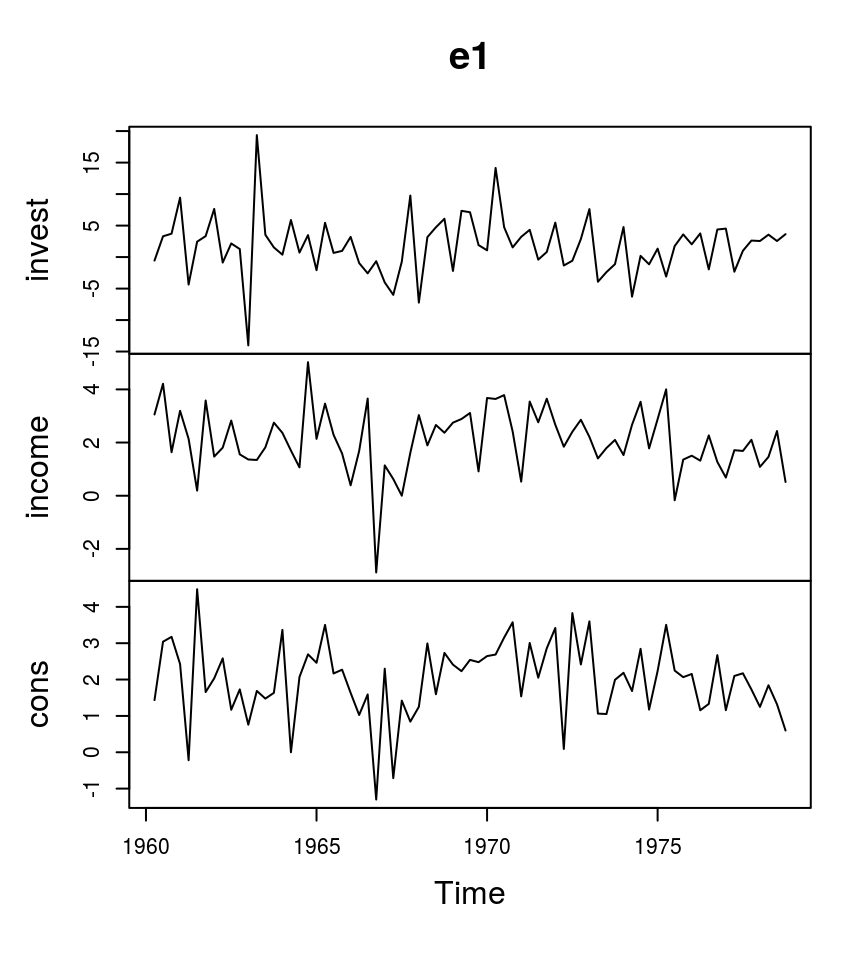
To assist with the set-up of the model the gen_var function produces the inputs y and x for the estimator, where y is a matrix of dependent variables and x is the matrix of regressors for the model
\[y_t = A x_t + u_t,\] with \(u_t \sim N(0, \Sigma)\). This is a more compact form of the model above, where the lags of the endogenous variables and the constant are already included in \(x_t\).
data <- gen_var(e1, p = 2, deterministic = "const")

y <- t(data$data$Y)
x <- t(data$data$Z)
Estimation
Frequentist estimator
We calculate frequentist VAR estimates using the standard formula \(y x' (x x')^{-1}\) to obtain a benchmark for the Bayesian estimator. The parameters are obtained by OLS:
A_freq <- tcrossprod(y, x) %*% solve(tcrossprod(x)) # Calculate estimates
round(A_freq, 3) # Round estimates and print
## invest.1 income.1 cons.1 invest.2 income.2 cons.2 const
## invest -0.320 0.146 0.961 -0.161 0.115 0.934 -1.672
## income 0.044 -0.153 0.289 0.050 0.019 -0.010 1.577
## cons -0.002 0.225 -0.264 0.034 0.355 -0.022 1.293And \(\Sigma\) is calculated by
u_freq <- y - A_freq %*% x
u_sigma_freq <- tcrossprod(u_freq) / (ncol(y) - nrow(x))
round(u_sigma_freq, 2)
## invest income cons
## invest 21.30 0.72 1.23
## income 0.72 1.37 0.61
## cons 1.23 0.61 0.89These are virtually the same values as in Lütkepohl (2007, Ch. 3). The only differences stem from the re-scaling of the data above, which results in proportionally higher values for the const variable and does not require us to multiply the covariance matrix by \(10^4\).
Bayesian estimator
The following code is a Gibbs sampler for a simple VAR model with non-informative priors. First, we define some variables, which help in the set-up of the sampler:
# Reset random number generator for reproducibility
set.seed(1234567)

iter <- 30000 # Number of iterations of the Gibbs sampler
burnin <- 15000 # Number of burn-in draws
store <- iter - burnin

tt <- ncol(y) # Number of observations
k <- nrow(y) # Number of endogenous variables
m <- k * nrow(x) # Number of estimated coefficients
Next, we set the priors. The prior means of the coefficient vector \(a = vec(A)\) are set to \(0\) and the diagonal elements of the corresponding covariance matrix \(V\) are set to \(1\), except for coefficients corresponding to intercept terms, which are set to \(10\). The prior degrees of freedom of the error term are set to \(6\) and the diagonal elements of the scale matrix to \(1\).
Note that the choice of the prior variances for coefficients, which correspond to intercept terms, can be motivated by the values of the analysed time series. For example, if a stationary series seems to move around the value \(5\), this could be taken into account by setting the prior mean of the respective coefficients to \(5\) with a small prior variance around it. If the researcher still prefers to set the mean to \(0\), it should be ensured that the prior variance is large enough so that the value \(5\) is captured by the prior distribution.
Note that the choice of the prior variances of the errors can be highly influential if the scale of the errors is not taken into account appropriately. For example, if the dependent variable does exceed values between \(-0.1\) and \(0.1\), a prior of \(1\) would be too high and could lead to useless results.
# Set priors
a_mu_prior <- matrix(0, m) # Vector of prior parameter means
a_v_i_prior <- diag(1, m) # Inverse of the prior covariance matrix

u_sigma_df_prior <- 6 # Prior degrees of freedom
u_sigma_scale_prior <- diag(1, k) # Prior covariance matrix
u_sigma_df_post <- tt + u_sigma_df_prior # Posterior degrees of freedom
Note that we could also use uninformative priors, where all elements of the inverse prior covariance matrix \(V^{-1}\) are set to zero and the prior degrees of freedom and the elements of the scale matrix are set to 0 as well. Such a specification should lead to posterior draws, which mimic the results of a frequentist OLS estimator.
Then we obtain some starting values. It might be a good idea to start with the OLS estimates of the model.
# Initial values
u_sigma_i <- solve(u_sigma_freq)
Next, create object, in which the posterior draws are saved for later.
# Data containers for posterior draws
draws_a <- matrix(NA, m, store)
draws_sigma <- matrix(NA, k * k, store)
Finally run the Gibbs sampler.
# Start Gibbs sampler
for (draw in 1:iter) {
  # Draw conditional mean parameters
  a <- post_normal(y, x, u_sigma_i, a_mu_prior, a_v_i_prior)

  # Draw variance-covariance matrix
  u <- y - matrix(a, k) %*% x # Obtain residuals
  u_sigma_scale_post <- solve(u_sigma_scale_prior + tcrossprod(u))
  u_sigma_i <- matrix(rWishart(1, u_sigma_df_post, u_sigma_scale_post)[,, 1], k)
  u_sigma <- solve(u_sigma_i) # Invert Sigma_i to obtain Sigma

  # Store draws
  if (draw > burnin) {
    draws_a[, draw - burnin] <- a
    draws_sigma[, draw - burnin] <- u_sigma
  }
}
After the Gibbs sampler has finished, point estimates for the coefficient matrix can be obtained as, e.g., the mean of the posterior draws:
A <- rowMeans(draws_a) # Obtain means for every row
A <- matrix(A, k) # Transform mean vector into a matrix
A <- round(A, 3) # Round values
dimnames(A) <- list(dimnames(y)[[1]], dimnames(x)[[1]]) # Rename matrix dimensions

A # Print
## invest.1 income.1 cons.1 invest.2 income.2 cons.2 const
## invest -0.284 0.200 0.573 -0.141 0.170 0.540 -0.353
## income 0.041 -0.132 0.327 0.048 0.036 0.035 1.307
## cons -0.003 0.237 -0.244 0.033 0.365 0.000 1.145Point estimates for the covariance matrix can also be obtained by calculating the means of the posterior draws.
Sigma <- rowMeans(draws_sigma) # Obtain means for every row
Sigma <- matrix(Sigma, k) # Transform mean vector into a matrix
Sigma <- round(Sigma, 2) # Round values
dimnames(Sigma) <- list(dimnames(y)[[1]], dimnames(y)[[1]]) # Rename matrix dimensions

Sigma # Print
## invest income cons
## invest 20.45 0.64 1.15
## income 0.64 1.35 0.59
## cons 1.15 0.59 0.88The means of the coefficient draws are relatively close to the results of the frequentist estimatior. However, note that the frequentist estimator suggests coefficients, which are close to \(1\) for the relationship between investment and consumption. By contrast, the Bayesian estimator implies different point estimates, which might be a result of the rather close prior variance of \(1\) for those parameters. As mentioned above, using a non-informative prior will lead to results that are closer to the OLS estimates.
bvar objects
The bvar function can be used to collect relevant output of the Gibbs sampler into a standardised object, which can be used by further functions such as predict to obtain forecasts or irf for impulse respons analysis.
bvar_est <- bvar(y = data$data$Y, x = data$data$Z, A = draws_a[1:18,],
                 C = draws_a[19:21, ], Sigma = draws_sigma)
There is also a summary function, which calculates some summary statistics
summary(bvar_est)##
## Model:
##
## y ~ invest.1 + income.1 + cons.1 + invest.2 + income.2 + cons.2 + const
##
## Variable: invest
##
## Mean SD Naive SD Time-series SD 2.5% 50% 97.5%
## invest.1 -0.2844 0.1201 0.0009808 0.0009808 -0.5211 -0.2840 -0.04532
## income.1 0.2002 0.4413 0.0036029 0.0035232 -0.6628 0.2007 1.05986
## cons.1 0.5730 0.4895 0.0039965 0.0039965 -0.3833 0.5736 1.52662
## invest.2 -0.1412 0.1213 0.0009908 0.0009746 -0.3800 -0.1424 0.09921
## income.2 0.1704 0.4332 0.0035367 0.0035367 -0.6717 0.1682 1.01781
## cons.2 0.5397 0.4883 0.0039868 0.0039868 -0.4246 0.5369 1.49972
## const -0.3535 0.8423 0.0068772 0.0068772 -1.9975 -0.3569 1.29657
##
## Variable: income
##
## Mean SD Naive SD Time-series SD 2.5% 50% 97.5%
## invest.1 0.04132 0.03153 0.0002575 0.0002455 -0.02041 0.04137 0.1027
## income.1 -0.13168 0.13447 0.0010980 0.0010936 -0.39691 -0.13156 0.1344
## cons.1 0.32719 0.15914 0.0012994 0.0012980 0.01486 0.32633 0.6412
## invest.2 0.04820 0.03159 0.0002579 0.0002579 -0.01474 0.04822 0.1110
## income.2 0.03612 0.13057 0.0010661 0.0010699 -0.22046 0.03603 0.2928
## cons.2 0.03473 0.16004 0.0013067 0.0013039 -0.27911 0.03425 0.3481
## const 1.30700 0.38809 0.0031687 0.0031687 0.54084 1.30723 2.0596
##
## Variable: cons
##
## Mean SD Naive SD Time-series SD 2.5% 50%
## invest.1 -0.0032834 0.02548 0.0002080 0.0002080 -0.05363 -0.0032451
## income.1 0.2366413 0.10776 0.0008799 0.0008932 0.02461 0.2361275
## cons.1 -0.2440363 0.12810 0.0010459 0.0010631 -0.49374 -0.2447420
## invest.2 0.0332773 0.02532 0.0002067 0.0002067 -0.01658 0.0334376
## income.2 0.3653053 0.10428 0.0008515 0.0008515 0.16126 0.3653724
## cons.2 0.0003121 0.12840 0.0010484 0.0010484 -0.25214 -0.0007522
## const 1.1448477 0.31103 0.0025396 0.0025396 0.52840 1.1449082
## 97.5%
## invest.1 0.046427
## income.1 0.446671
## cons.1 0.005891
## invest.2 0.082497
## income.2 0.572533
## cons.2 0.251092
## const 1.755069
##
## Variance-covariance matrix:
##
## Mean SD Naive SD Time-series SD 2.5% 50% 97.5%
## invest_invest 20.4491 3.5030 0.028602 0.030332 14.6936 20.0350 28.3671
## invest_income 0.6355 0.6416 0.005239 0.005635 -0.5924 0.6194 1.9571
## invest_cons 1.1484 0.5294 0.004323 0.004630 0.1991 1.1213 2.2745
## income_invest 0.6355 0.6416 0.005239 0.005635 -0.5924 0.6194 1.9571
## income_income 1.3486 0.2357 0.001925 0.002131 0.9656 1.3221 1.8823
## income_cons 0.5947 0.1516 0.001238 0.001359 0.3383 0.5815 0.9311
## cons_invest 1.1484 0.5294 0.004323 0.004630 0.1991 1.1213 2.2745
## cons_income 0.5947 0.1516 0.001238 0.001359 0.3383 0.5815 0.9311
## cons_cons 0.8770 0.1527 0.001246 0.001382 0.6252 0.8609 1.2227Posterior draws can be thinned with the function thin:
bvar_est <- thin_posterior(bvar_est, thin = 15)Forecasts
Forecasts with credible bands can be obtained with the function predict. If the model contains deterministic terms, new values can be provided in the argument new_d. If no values are provided, the function sets them to zero. The number of rows of new_d must be the same as the argument n.ahead.
bvar_pred <- predict(bvar_est, n.ahead = 10, new_d = rep(1, 10))

plot(bvar_pred)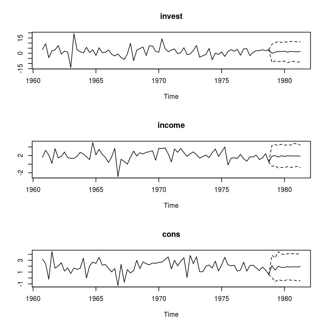
Impulse response analysis
Currently, bvartools supports forecast error, orthogonalised, and generalised impulse response functions.
Forecast error impulse response
FEIR <- irf(bvar_est, impulse = "income", response = "cons", n.ahead = 8)

plot(FEIR, main = "Forecast Error Impulse Response", xlab = "Period", ylab = "Response")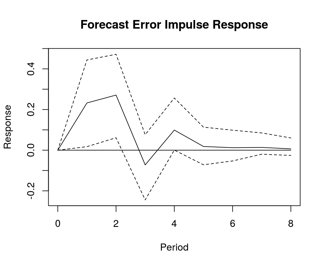
Orthogonalised impulse response
OIR <- irf(bvar_est, impulse = "income", response = "cons", n.ahead = 8, type = "oir")

plot(OIR, main = "Orthogonalised Impulse Response", xlab = "Period", ylab = "Response")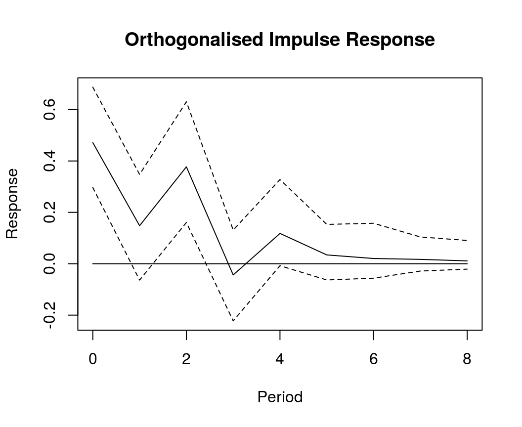
Generalised impulse response
GIR <- irf(bvar_est, impulse = "income", response = "cons", n.ahead = 8, type = "gir")

plot(GIR, main = "Generalised Impulse Response", xlab = "Period", ylab = "Response")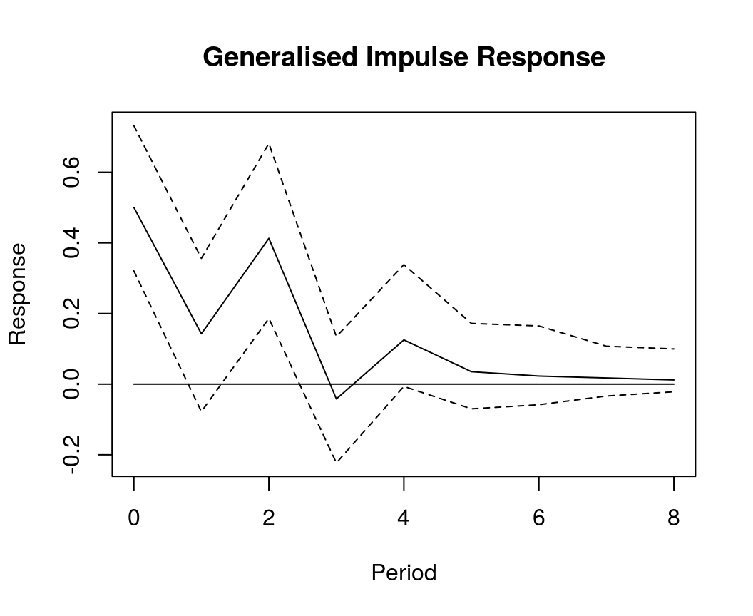
Forecast error variance decomposition
Default forecast error variance decomposition (FEVD) is based on orthogonalised impulse responses (OIR).
bvar_fevd_oir <- fevd(bvar_est, response = "cons")

plot(bvar_fevd_oir, main = "OIR-based FEVD of consumption")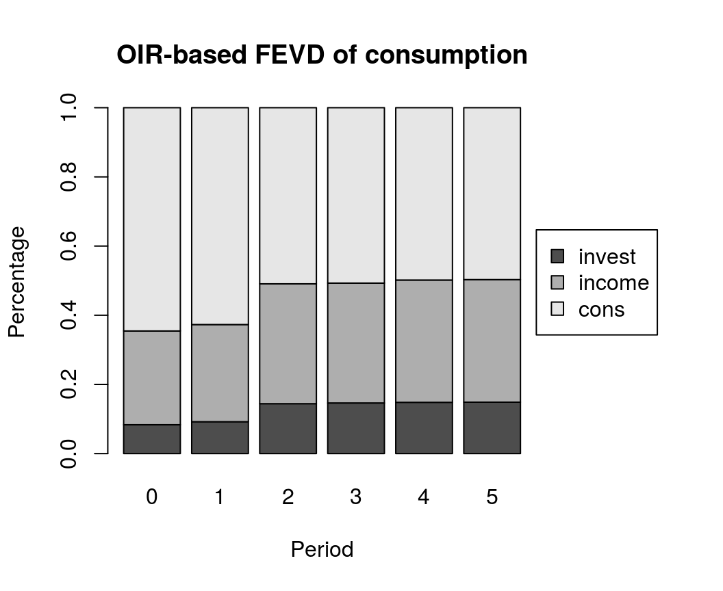
It is also possible to calculate FEVDs, which are based on generalised impulse responses (GIR). Note that these do not automatically add up to unity.
bvar_fevd_gir <- fevd(bvar_est, response = "cons", type = "gir")

plot(bvar_fevd_gir, main = "GIR-based FEVD of consumption")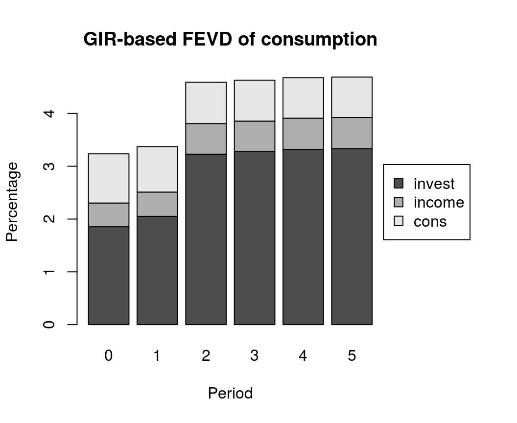
References
Chan, J., Koop, G., Poirier, D. J., & Tobias, J. L. (2019). Bayesian Econometric Methods (2nd ed.). Cambridge: University Press.
Koop, G., & Korobilis, D. (2010). Bayesian multivariate time series methods for empirical macroeconomics. Foundations and trends in econometrics, 3(4), 267-358. https://dx.doi.org/10.1561/0800000013
Koop, G., Pesaran, M. H., & Potter, S.M. (1996). Impulse response analysis in nonlinear multivariate models. Journal of Econometrics 74(1), 119-147. https://doi.org/10.1016/0304-4076(95)01753-4
Lütkepohl, H. (2007). New introduction to multiple time series analysis (2nd ed.). Berlin: Springer.
Kennedy, P. (2008). A guide to econometrics (6th ed.) Malden, MA: Blackwell.
Pesaran, H. H., & Shin, Y. (1998). Generalized impulse response analysis in linear multivariate models. Economics Letters, 58(1), 17-29. https://doi.org/10.1016/S0165-1765(97)00214-0