Bayesian Error Correction Models with Priors on the Cointegration Space
with tags r bvec vec cointegration bvartools -Introduction
This post provides the code to set up and estimate a basic Bayesian vector error correction (BVEC) model with the bvartools package. The presented Gibbs sampler is based on the approach of Koop et al. (2010), who propose a prior on the cointegration space.
Data
To illustrate the estimation process, the dataset E6 from Lütkepohl (2007) is used, which contains data on German long-term interest rates and inflation from 1972Q2 to 1998Q4.
library(bvartools)

data("e6")

plot(e6) # Plot the series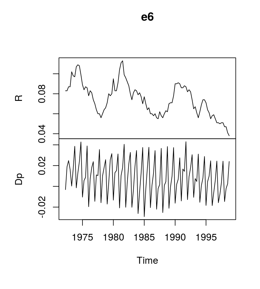
The gen_vec function produces the inputs Y, W and X for the BVEC estimator, where Y is the matrix of dependent variables, W is a matrix of potentially cointegrated regressors, and X is the matrix of non-cointegration regressors.
data <- gen_vec(e6, p = 4, r = 1, const = "unrestricted", season = "unrestricted")

y <- t(data$data$Y)
w <- t(data$data$W)
x <- t(data$data$X)
Estimation
# Reset random number generator for reproducibility
set.seed(7654321)

iter <- 10000 # Number of iterations of the Gibbs sampler
burnin <- 5000 # Number of burn-in draws
store <- iter - burnin

r <- 1 # Set rank

t <- ncol(y) # Number of observations
k <- nrow(y) # Number of endogenous variables
k_w <- nrow(w) # Number of regressors in error correction term
k_x <- nrow(x) # Number of differenced regressors and unrestrictec deterministic terms

k_alpha <- k * r # Number of elements in alpha
k_beta <- k_w * r # Number of elements in beta
k_gamma <- k * k_x

# Set uninformative priors
# ...for non-cointegration parameters
a_mu_prior <- matrix(0, k_x * k) # Vector of prior parameter means
a_v_i_prior <- diag(0, k_x * k) # Inverse of the prior covariance matrix

# ...for cointegration parameters
v_i <- 0
p_tau_i <- matrix(0, k_w, k_w)
p_tau_i[1:r, 1:r] <- diag(1, r)

#...for the error term
u_sigma_df_prior <- r # Prior degrees of freedom
u_sigma_scale_prior <- diag(0, k) # Prior covariance matrix
u_sigma_df_post <- t + u_sigma_df_prior # Posterior degrees of freedom

# Initial values
beta <- matrix(c(1, -4), k_w, r)

u_sigma_i <- diag(.0001, k)
u_sigma <- solve(u_sigma_i)

g_i <- u_sigma_i

# Data containers
draws_alpha <- matrix(NA, k_alpha, store)
draws_beta <- matrix(NA, k_beta, store)
draws_pi <- matrix(NA, k * k_w, store)
draws_gamma <- matrix(NA, k_gamma, store)
draws_sigma <- matrix(NA, k^2, store)

# Start Gibbs sampler
for (draw in 1:iter) {
  # Draw conditional mean parameters
  temp <- post_coint_kls(y = y, beta = beta, w = w, x = x, sigma_i = u_sigma_i,
                           v_i = v_i, p_tau_i = p_tau_i, g_i = g_i,
                           gamma_mu_prior = a_mu_prior,
                           gamma_v_i_prior = a_v_i_prior)
  alpha <- temp$alpha
  beta <- temp$beta
  Pi <- temp$Pi
  gamma <- temp$Gamma

  # Draw variance-covariance matrix
  u <- y - Pi %*% w - matrix(gamma, k) %*% x
  u_sigma_scale_post <- solve(tcrossprod(u) + v_i * alpha %*% tcrossprod(crossprod(beta, p_tau_i) %*% beta, alpha))
  u_sigma_i <- matrix(rWishart(1, u_sigma_df_post, u_sigma_scale_post)[,, 1], k)
  u_sigma <- solve(u_sigma_i)

  # Update g_i
  g_i <- u_sigma_i

  # Store draws
  if (draw > burnin) {
    draws_alpha[, draw - burnin] <- alpha
    draws_beta[, draw - burnin] <- beta
    draws_pi[, draw - burnin] <- Pi
    draws_gamma[, draw - burnin] <- gamma
    draws_sigma[, draw - burnin] <- u_sigma
  }
}
Obtain point estimates as the mean of the parameter draws:
Gamma <- rowMeans(draws_gamma) # Obtain means for every row
Gamma <- matrix(Gamma, k) # Transform mean vector into a matrix
Gamma <- round(Gamma, 3) # Round values
dimnames(Gamma) <- list(dimnames(y)[[1]], dimnames(x)[[1]]) # Rename matrix dimensions

round(Gamma, 3) # Print
## d.R.l1 d.Dp.l1 d.R.l2 d.Dp.l2 d.R.l3 d.Dp.l3 const season.1 season.2
## d.R 0.267 -0.187 -0.017 -0.207 0.225 -0.099 0.002 0.001 0.009
## d.Dp 0.074 -0.383 0.000 -0.421 0.025 -0.361 0.011 -0.034 -0.018
## season.3
## d.R 0.000
## d.Dp -0.017beta <- rowMeans(t(t(draws_beta) / t(draws_beta)[, 1])) # Obtain means for every row
beta <- matrix(beta, k_w) # Transform mean vector into a matrix
beta <- round(beta, 3) # Round values
dimnames(beta) <- list(dimnames(w)[[1]], NULL) # Rename matrix dimensions
beta # Print## [,1]
## l.R 1.000
## l.Dp -3.969Sigma <- rowMeans(draws_sigma) # Obtain means for every row
Sigma <- matrix(Sigma, k) # Transform mean vector into a matrix
Sigma <- round(Sigma * 10^4, 2) # Round values
dimnames(Sigma) <- list(dimnames(y)[[1]], dimnames(y)[[1]]) # Rename matrix dimensions
Sigma # Print## d.R d.Dp
## d.R 0.29 -0.02
## d.Dp -0.02 0.27bvec objects
The bvec function can be used to collect output of the Gibbs sampler in a standardised object, which can be used further for forecasting, impulse response analysis or forecast error variance decomposition.
# Number of non-deterministic coefficients
k_nondet <- (k_x - 4) * k

# Generate bvec object
bvec_est <- bvec(y = data$data$Y, w = data$data$W,
                 x = data$data$X[, 1:6],
                 x_d = data$data$X[, 7:10],
                 Pi = draws_pi,
               Gamma = draws_gamma[1:k_nondet,],
               C = draws_gamma[(k_nondet + 1):nrow(draws_gamma),],
               Sigma = draws_sigma)
Posterior draws can be thinned with function thin:
bvec_est <- thin_posterior(bvec_est, thin = 5)The function bvec_to_bvar can be used to transform the VEC model into a VAR in levels:
bvar_form <- bvec_to_bvar(bvec_est)Forecasts
bvar_pred <- predict(bvar_form, n.ahead = 10, new_d = bvar_form$x[3 + 1:10, 9:12])

plot(bvar_pred)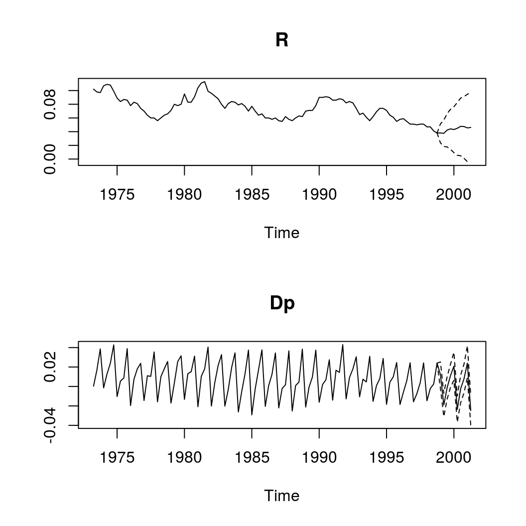
Impulse response analysis
Impulse responses for VECs can be constructed from their VAR respresentations.
IR <- irf(bvar_form, impulse = "R", response = "Dp", n.ahead = 20)

plot(IR, main = "Forecast Error Impulse Response", xlab = "Year", ylab = "Response")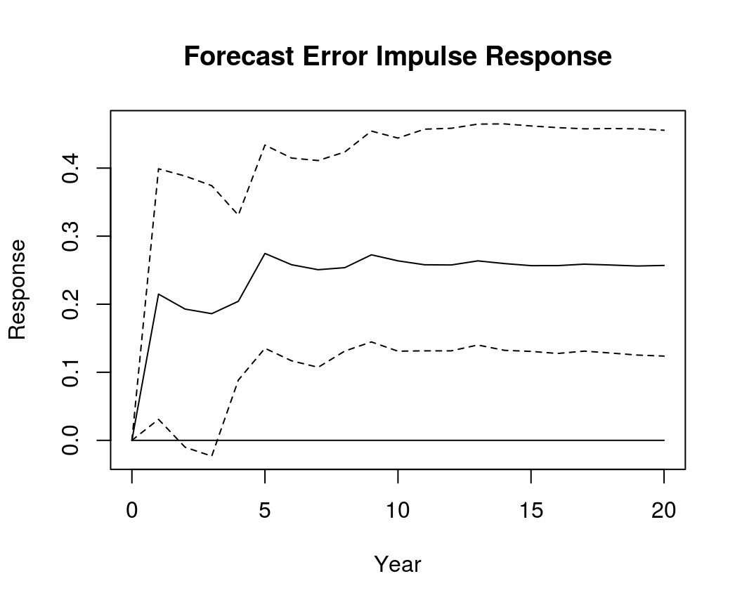
Orthogonalised impulse response
OIR <- irf(bvar_form, impulse = "R", response = "Dp", n.ahead = 20, type = "oir")

plot(OIR, main = "Orthogonalised Impulse Response", xlab = "Year", ylab = "Response")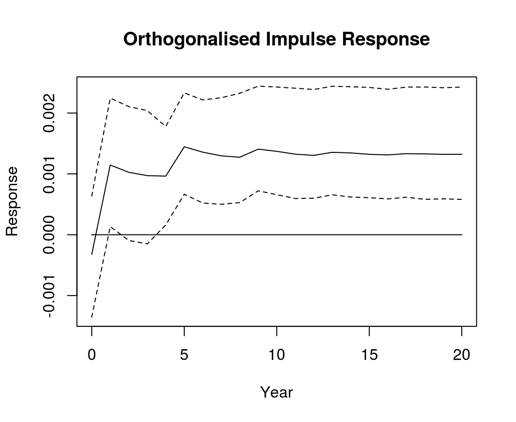
Generalised impulse response
GIR <- irf(bvar_form, impulse = "R", response = "Dp", n.ahead = 20, type = "gir")

plot(GIR, main = "Generalised Impulse Response", xlab = "Year", ylab = "Response")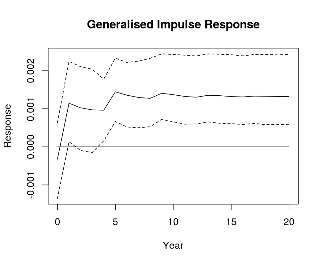
Forecast error variance decomposition
bvec_fevd <- fevd(bvar_form, response = "Dp", n.ahead = 20)

plot(bvec_fevd, main = "FEVD of inflation")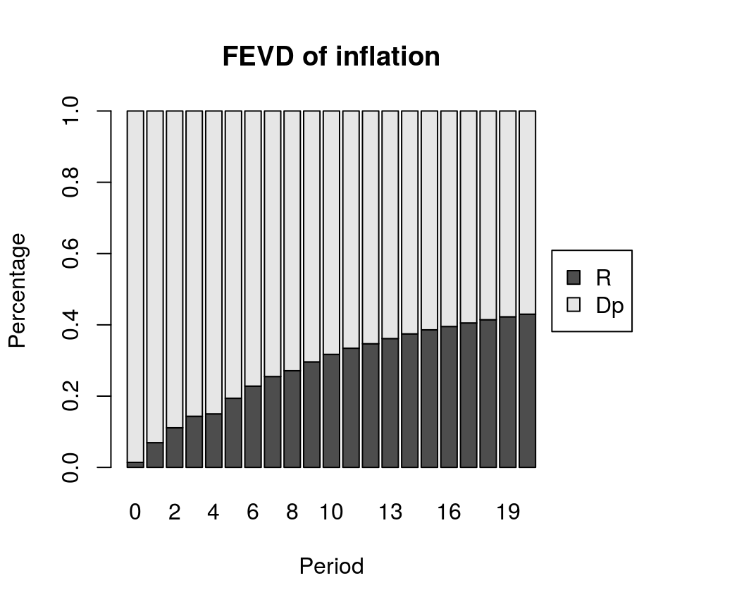
References
Koop, G., León-González, R., & Strachan R. W. (2010). Efficient posterior simulation for cointegrated models with priors on the cointegration space. Econometric Reviews, 29(2), 224-242. https://doi.org/10.1080/07474930903382208
Lütkepohl, H. (2007). New introduction to multiple time series analysis (2nd ed.). Berlin: Springer.
Pesaran, H. H., & Shin, Y. (1998). Generalized impulse response analysis in linear multivariate models, Economics Letters, 58, 17-29. https://doi.org/10.1016/S0165-1765(97)00214-0