An Introduction to Dynamic Factor Models

Introduction

For some macroeconomic applications it might be interesting to see whether a set of obserable variables depends on common drivers. The estimation of such common factors can be done using so-called factor analytical models, which have the form

\[x_t = \lambda f_t + u_t,\]

where \(x_t\) is an \(M\)-dimensional vector of observable variables, \(f_t\) is an \(N \times 1\) vector of unobserved factors, \(\lambda\) is an \(M \times N\) matrix of factor loadings and \(u_t\) is an error term.

The above model is static in the sense that it does not allow for autocorrelation of the factors. However, for time series applications it is common to model the factors by assuming an autoregressive process:

\[f_t = A_1 f_{t-1} + ... + A_p f_{t-p} + v_t,\] where \(A_i\) is the \(N \times N\) coefficient matrix correponding to the \(i\)th lag of factor \(f_t\) and \(v_t\) is an error term. This makes the model more dynamic and, hence, the approach is called dynamic factor model (DFM).

A basic DFM consists of two equation: First, the measurement equation (the first equation above), which describes the relationship between the observed variables and the factors. Second, the transition equation (the second equation above) describing the intertemporal relationships between the factors.¹

To ensure that DMFs can be estiamted from a mathematical perspective, some identifying assumptions need to be made. A popular approach is to assume that the covariance matrices of the error terms \(u_t\) and \(v_t\) are diagonal, so that they only include the variances of the variables. Furthermore, the matrix of factor loadings \(\lambda\) is assumed to be lower triangular with ones on the main diagonal. For example, the measurement equation of a DFM with \(M\) observable variables and 2 factors could be written as:

\[ \begin{pmatrix} x_{1,t} \\ x_{2,t} \\ x_{3,t} \\ \vdots \\ x_{M,t} \end{pmatrix} = \begin{bmatrix} 1 & 0 \\ \lambda_{21} & 1 \\ \lambda_{31} & \lambda_{32} \\ \vdots & \vdots \\ \lambda_{M1} & \lambda_{M2} \end{bmatrix} \begin{pmatrix} f_{1,t} \\ f_{2,t} \end{pmatrix} + u_t \] with \(u_t \sim N(0, \Sigma_u)\) and \[\Sigma_u = \begin{bmatrix} \sigma_{u, 11}^{2} & 0 & \dots & 0 \\ 0 & \sigma_{u, 22}^{2} & \ddots & \vdots \\ \vdots & \ddots & \ddots & \vdots \\ 0 & \dots & \dots & \sigma_{u, MM}^{2} \end{bmatrix}.\]

The corresponding transistion equation would have the usual form of a VAR(\(p\)) with \(v_t \sim N(0, \Sigma_v)\) and \(\Sigma_v = \begin{bmatrix} \sigma_{v, 11}^{2} & 0 \\ 0 & \sigma_{v, 22}^{2} \end{bmatrix}.\)

Application

Since version 0.2.0 the bvartoolspackage can be used to estimate dynamic factor models as described above using Bayesian inference. The implementation follows the Matlab code privided in the online annex to the textbook of Chan, Koop, Poirier and Tobias (2019). The following application is a reproduction of exercise 18.4 in the textbook, where quarterly time series data on 196 macroeconomic variables is used to extract a common factor for the US. The prepared data set is contained in the package.

# Load package
library(bvartools)

# Load data
data("bem_dfmdata")

Following the logic of the bvartools package, the estimation process is divided into four parts. First, using gen_dfm an object is created, which contains all information required by the estimation algorithm. For the current application we set the number of factors to 1 and the number of lags in the transition equation to 1 as well.

# Generate input for estimation
object <- gen_dfm(x = bem_dfmdata, p = 1, n = 1, iterations = 5000, burnin = 1000)

Second, add_priors is used to add prior information to the model object. We use the same priors that as in Chan et al. (2019).

# Priors
object <- add_priors(object,
                     lambda = list(v_i = .01),
                     a = list(v_i = .01),
                     sigma_v = list(shape = 5, rate = 4),
                     sigma_u = list(shape = 5, rate = 4))

Third, we obtain posterior draws, where the researcher can either implement her own algorithm or use the simple Gibbs sampler that comes with the package. For this application, the built-in sampler is used:

# Procude posterior draws
object <- draw_posterior(object)

## Estimating models...

Forth, evaluate the results. Currently, the package only allows to plot the factors:

plot(object)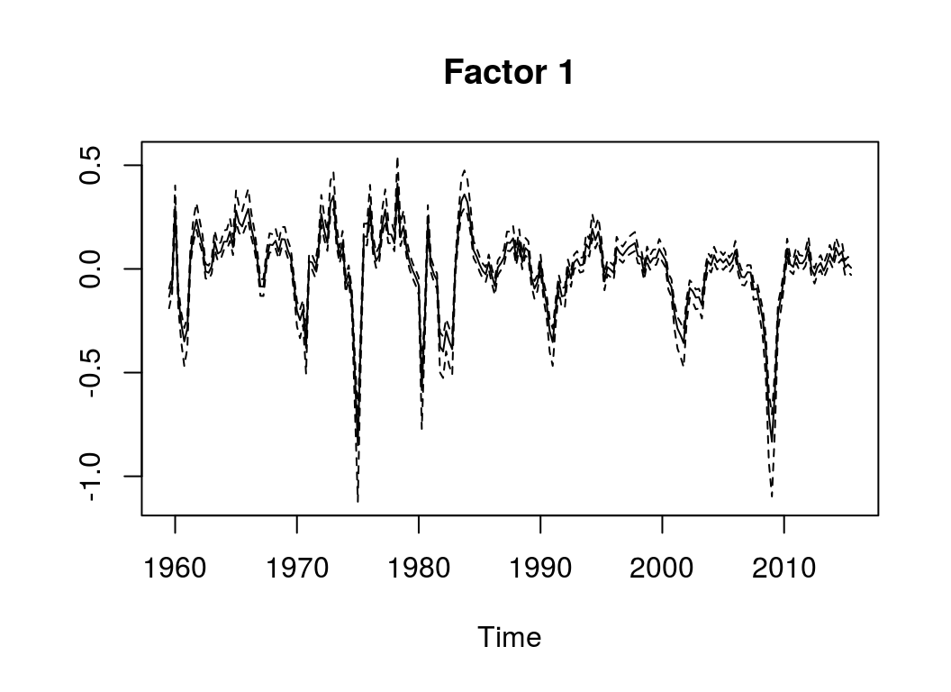

References

Chan, J., Koop, G., Poirier, D. J., & Tobias, J. L. (2019). Bayesian Econometric Methods (2nd ed.). Cambridge: University Press.

Lütkepohl, H. (2007). New introduction to multiple time series analysis (2nd ed.). Berlin: Springer.