Extracting Cyclical Components From Economic Time Series

Data

I use quarterly data of US log real GDP from 1970Q1 to 2016Q4 for the illustration of the different methods. The time series is obtained via Quandl and its respectiv R-package. The original series can be downloaded from the FRED database.

# Load packages for data download and transformation
library(dplyr)
library(Quandl)
library(tidyr)

# Download data
data <- Quandl("FRED/GDPC1", order = "asc",
               start_date = "1970-01-01", end_date = "2016-10-01")  %>%
  rename(date = Date,
         gdp = Value) %>%
  mutate(lgdp = log(gdp)) # Take logs

To get an intuition about what it means to extract the cyclical component of a time series, look at the development of log real GDP over time in the following figure.

library(ggplot2)

ggplot(data, aes(x = date, y = lgdp)) +
  geom_line() +
  theme_classic() +
  labs(title = "Log real US GDP", x = "Quarter", y = "",
       caption = "Source: U.S. Bureau of Economic Analysis (GDPC1).\nRetrieved via Quandl.com.")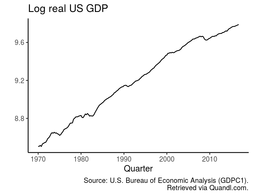

There is a clear increasing trend in the data, which appears to become gradually smaller up to the present. Additionally, the series seems to fluctuate around this trend in a more or less regular manner. There are relatively long lasting deviations from the trend, which could be considered to be cyclical fluctuations. The identification of those cyclical components is an important question in economics, because it might have serious implications for economic policy.

Deviation from a linear trend

A first approach to extract a trend from a series is to regress the variable of interest on a constant and a trend term and to obtain the fitted values. These are plotted in the following figure.

# Add a trend
data <- data %>%
  mutate(trend = 1:n())

# Estimate the model with a constant and a trend
time_detrend <- fitted(lm(lgdp ~ trend, data = data))
names(time_detrend) <- NULL

# Add series to main data frame
data <- data %>%
  mutate(lin_trend = time_detrend)

# Create data frame for the plot
temp <- data %>%
  select(date, lgdp, lin_trend) %>%
  gather(key = "Variable", value = "value", -date)

# Plot
ggplot(temp, aes(x = date, y = value, colour = Variable)) +
  geom_line() +
  theme_classic() +
  labs(title = "Residuals of a linear trend estimation",
       x = "Quarter", y = "")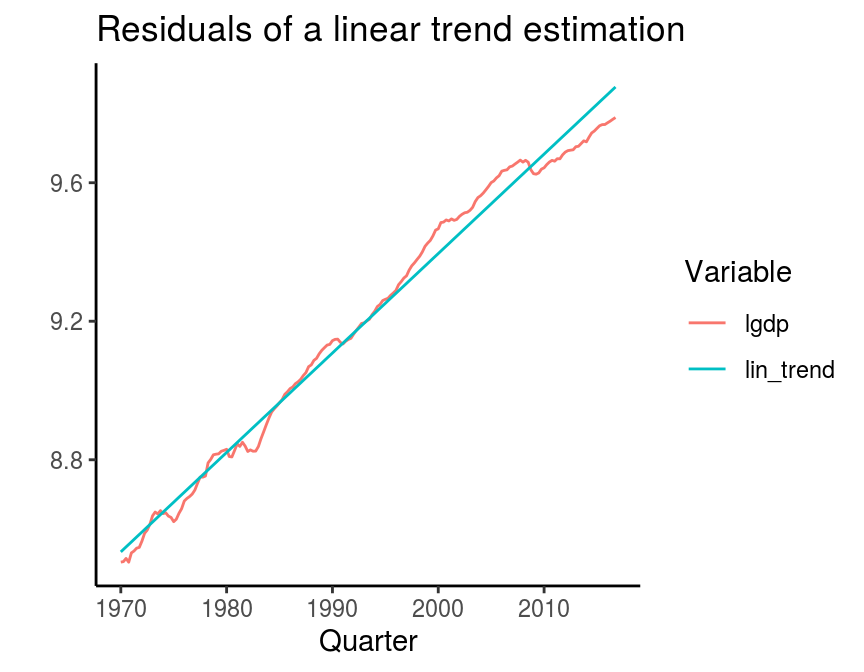

This approach is relatively controversial, since it assumes that there is a constant, linear time trend. As we have seen above, this is not very likely given the steady decrease of the trend’s growth rate over time. However, it is still possible to assume a different functional form of the time trend, e.g. a quadratic term, to account for the specifities of a trend. A further disadvantage of this method is that it does only exlude the trend, but not the noise, i.e. the very small fluctuations in the series.

Hodrick-Prescott filter

Hodrick and Prescott (1981) developed a filter, which seprates a time series into a trend and cyclical component. In contrast to the linear trend the so-called HP filter estimates a trend, which changes over time. And the degree to which this trend is allowed to change, the smoothing parameter \(\lambda\), is determined manually by the researcher.

The hpfilter function is contained in the mFilter package and requires the time series and the smoothing parameter. The literature suggests a value of 1600 for quarterly data. However, it is possible to choose a much higher value as well. The follwoing figure plots the values of the cyclical component of real GDP obtained by the HP filter and compares it to the values of a linearly detrended series. The behaviour of both series appears to be quite similar at the beginning of the series.

# Load the package
library(mFilter)

# Run HP filter
hp_gdp <- hpfilter(data$lgdp, freq = 1600)

# Add the cyclical component of the HP filter and
# the linearly detrended sereis to the main data frame
data <- data %>%
  mutate(hp = hp_gdp$cycle,
         lin_cycle = lgdp - lin_trend)

# Create data frame for the plot
temp <- data %>%
  select(date, hp, lin_cycle) %>%
  gather(key = "Variable", value = "value", -date) %>%
  filter(!is.na(value)) %>%
  mutate(Variable = factor(Variable, levels = c("hp", "lin_cycle"),
                           labels = c("HP filter", "Residuals of\na linear trend\nestimation")))

# Plot
ggplot(temp, aes(x = date, y = value, colour = Variable)) +
  geom_hline(yintercept = 0, colour = "grey") +
  geom_line() +
  theme_classic() +
  labs(title = "HP filter",
       x = "Qurarter", y = "")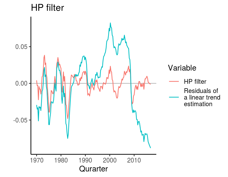

Although widely used in economics, the HP filter is also heavily criticised for some features. See, for example, a good overview in a Bruegel blog post by Jérémie Cohen-Setton and Yury Yatsynovich and here for the working paper version of a critique by James Hamilton.

A regression based alternative to the HP filter

Hamilton (2018) also proposes an alternative approach to the HP filter It boils down to a simple regression model, where the hth lead of the times series is regressed on the most recent p values of the time series. As recommended in the paper I use \(h = 8\) and \(p = 4\) in the following example. The package neverhpfilter by Justin M. Shea contains the function yth_filter, which requires an xts object as input.

library(neverhpfilter)

# Get the series
y <- as.xts(ts(data$lgdp, start = 1970, frequency = 4))

# Dimnames must be specified, otherwise the function won't accept the input
dimnames(y) <- list(NULL, "log_gdp")

# Estimate
hamilton_temp <- yth_filter(y, h = 8, p = 4)

# Add residuals to the main data frame
data <- data %>%
  mutate(hamilton = as.numeric(hamilton_temp$log_gdp.cycle))

# Prepare dataset for plot
temp <- data %>%
  select(date, hamilton, hp) %>%
  gather(key = "Variable", value = "value", -date) %>%
  filter(!is.na(value)) %>%
  mutate(Variable = factor(Variable,
                           levels = c("hp", "hamilton"),
                           labels = c("HP filter", "Hamilton's\nalternative\nto the HP-filter")))

# Plot
ggplot(temp, aes(x = date, y = value, colour = Variable)) +
  geom_hline(yintercept = 0, colour = "grey") +
  geom_line() +
  theme_classic() +
  labs(title = "Hamilton's alternative to the HP filter",
       x = "Qurarter", y = "", 
       caption = "Source: Hamilton (2018).")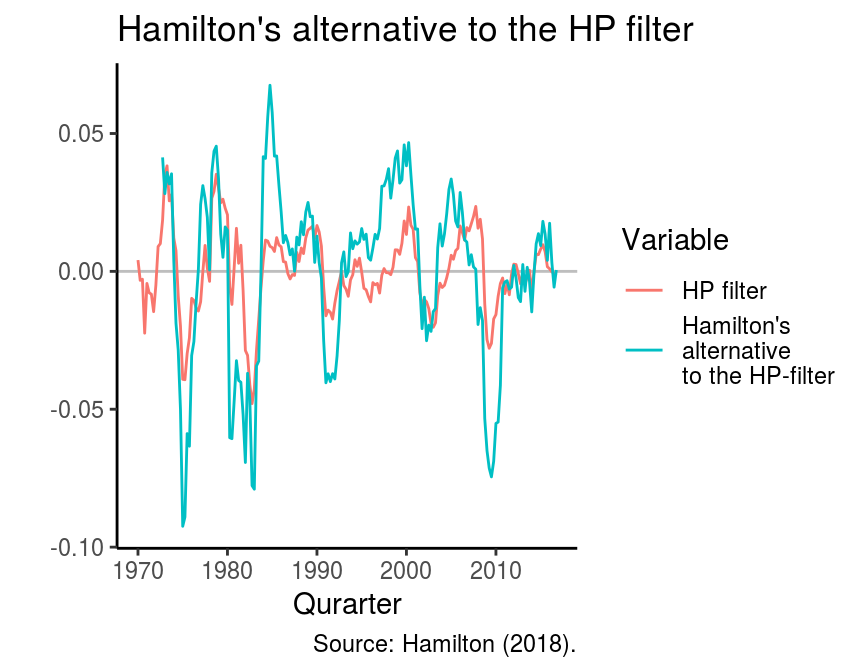

Baxter King filter

Baxter and King (1994, 1999) proposed a filter, which yields very similar results as the HP filter. Additionally, it takes out the noise from the time series, so that a smooth estimate of the cyclical component can be obtained. The function bkfilter is also contained in the mFilter package. It requires the series, a lower and an upper bound of the amount of periods, where cycles are assumed to occur (pl and pu), and a smoothing factor nfix. The literature (e.g. NBER, Stock and Watson (1999)) suggests that business cycles last from 6 to 32 months. These values were used to specify the lower and upper bound of the cycle periodicity. The results of the BK filter are shown in the following figure. A relatively serious drawback of this method is that the smoothing factor leads to the loss of observations at the beginning and the end of the series. This might be a problem with small samples and when the current state of the economy is of interest.

# Run BK filter
bk_gdp <- bkfilter(data$lgdp, pl = 6, pu = 32, nfix = 12)

# Add cyclical component to the main data frame
data <- data %>%
  mutate(bk = bk_gdp$cycle[, 1])

# Create data frame for the plot
temp <- data %>%
  select(date, hp, bk) %>%
gather(key = "Variable", value = "value", -date) %>%
  filter(!is.na(value)) %>%
  mutate(Variable = factor(Variable,
                           levels = c("hp", "bk"),
                           labels = c("HP filter", "BK filter")))

# Plot
ggplot(temp, aes(x = date, y = value, colour = Variable)) +
  geom_hline(yintercept = 0, colour = "grey") +
  geom_line() +
  theme_classic() +
  labs(title = "Baxter-King filter",
       x = "Qurarter", y = "")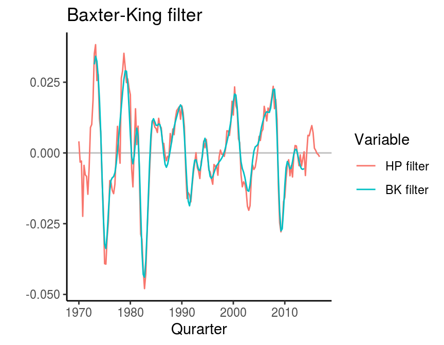

Wavelet filter

Yogo (2008) proposed to use wavelet filters to extract business cycles from time series data. The advantage of this method is that the function does not only allow to extract the trend, cycle and noise of a series, but also to become more specific about the periods within which cycles occur. However, there is not full freedom in that, since the technique can only capture periodicities of a power of two, i.e. 2, 4, 8, 16, 32 and so on.

The methods implementation in R is also neat, but requires some additional data transformation before it can be used. A useful function is contained in the waveslim package and is called mra (“multiresolution analysis”). It requires a differenced version of the time series and the depth of the decomposition.

# Load package
library(waveslim)

# Calculate first difference of log GDP
data <- data %>%
  mutate(dlgdp = lgdp - lag(lgdp, 1))

# Get data
y <- na.omit(data$dlgdp)

# Run the filter
wave_gdp <- mra(y, J = 5)

# Transform mra-output to data frame
wave_gdp <- as_tibble(wave_gdp)

# Create data frame for plotting
temp <- wave_gdp %>%
  gather(key = "imf", value = "value") %>%
  group_by(imf) %>%
  mutate(date = data$date[-1])

# Plot mra output
ggplot(temp, aes(x = date, y = value)) +
  geom_line() +
  facet_wrap( ~ imf, scales = "free") +
  labs(title = "Wavelets",
       x = "Quarter", y = "")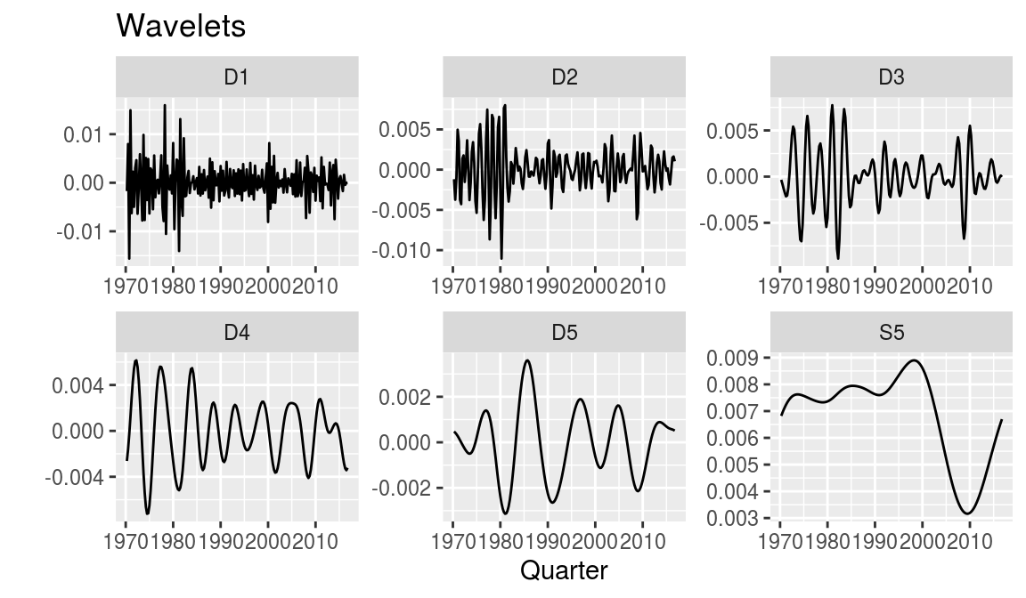

The function gives multiple series, which have to be cumulated with cumsum to translate them back into the level data. Maybe not surprisingly, the wavelet filter yields a similar result as the BK filter, since the upper bound of cycle periods is equal in both and the lower bound differs only by two - \(2^3 = 8\) compared to the \(6\) in the BK filter.

data <- data %>%
  mutate(wave = c(NA, cumsum(wave_gdp$D3 + wave_gdp$D4 + wave_gdp$D5)))

temp <- data %>%
  select(date, bk, wave) %>%
  gather(key = "Variable", value = "value", -date) %>%
  filter(!is.na(value)) %>%
  mutate(Variable = factor(Variable, levels = c("bk", "wave"),
                           labels = c("BK filter", "Wavelets")))

ggplot(temp, aes(x = date, y = value, colour = Variable)) +
  geom_hline(yintercept = 0, colour = "grey") +
  geom_line() +
  theme_classic() +
  labs(title = "Wavelets",
       x = "Quarter", y = "")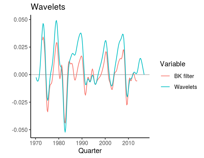

Empirical mode decomposition (EMD)

Kozic and Sever (2014) propose empirical mode decomposition as a further method of business cycle extraction as presented in Huang et al. (1998). An implementation of the method comes with the emd function in the EMD package. It requires a time series, which can be both stationary or non-stationary and a boundary condition. The basic idea of EMD is similar to wavelets. It decomposes a time series into sub-series, which are called intrinsic mode functions (IMF).

library(EMD)

y <- na.omit(data$lgdp)

# Run EMD
emd_gdp <- emd(xt = y, boundary = "none")

# Exctract the intrinsic mode functions
imf_gdp <- as.data.frame(emd_gdp$imf)

# Create a data frame for plotting
temp <- imf_gdp %>%
  gather(key = "imf", value = "value") %>%
  group_by(imf) %>%
  mutate(date = data$date)

# Plot the EMD output
ggplot(temp, aes(x = date, y = value)) +
  geom_line() +
  facet_wrap( ~ imf) +
  labs(title = "Empirical mode decomposition",
       x = "Quarter", y = "")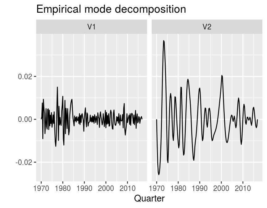

# Add EMD output to main data frame
data <- data %>%
  mutate(emd = lgdp - emd_gdp$residue)

# Create data frame for plotting
temp <- data %>%
  select(date, hp, emd) %>%
  gather(key = "Variable", value = "value", -date) %>%
  filter(!is.na(value)) %>%
  mutate(Variable = factor(Variable, levels = c("hp", "emd"),
                           labels = c("HP filter", "EMD")))

# Plot
ggplot(temp, aes(x = date, y = value, colour = Variable)) +
  geom_hline(yintercept = 0, colour = "grey") +
  geom_line() +
  theme_classic() +
  labs(title = "Empirical mode decomposition",
       x = "Qurarter", y = "")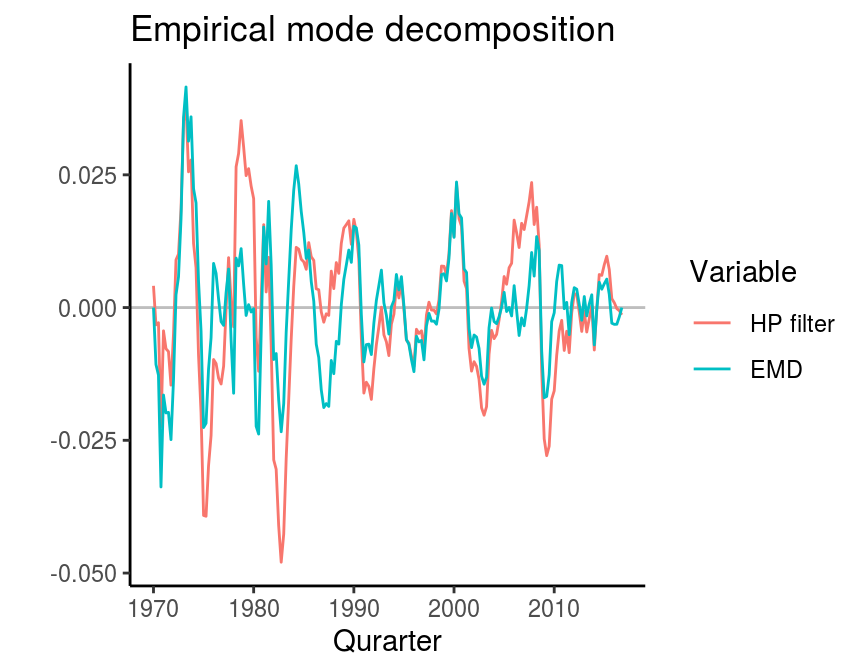

Note that the first and last elements are equal to zero. This is because we used the argument boundary = "none". If we used a different specification, the function would eliminate this boundary effect by extending the original series.

Grant, A. L., & Chan, J. C. C. (2017)

The followning code follows the description in Chan et al. (2019). The MATLAB code can be found on the textbook’s website.

Priors

# Rescaled data
y <- na.omit(data$lgdp) * 100
tt <- length(y) # T
p <- 2 # Lags of phi

# Priors of phi
prior_phi_mu <- matrix(c(1.3, -.7))
prior_phi_v_i <- diag(1, p)

# Priors of gamma
prior_gamma_mu <- matrix(c(850, 850)) # Should be close to first value of the series
prior_gamma_v_i <- diag(1 / 100, p)

# Priors for sigma2_tau
prior_s_tau <- .01

# Priors for sigma2_c
prior_s_c_shape <- 3
prior_s_c_rate <- 2

Initial values

# X_gamma
x_gamma <- cbind(2:(tt + 1), -1:-tt)

# H_2
h2 <- diag(1, tt)
diag(h2[-1, -tt]) <- -2
diag(h2[-(1:2), -((tt - 1):tt)]) <- 1
h2h2 <- crossprod(h2)

# H_phi
h_phi <- diag(1, tt)
phi <- matrix(c(1.34, -.7))
for (i in 1:p) {
  diag(h_phi[-(1:i), -((tt - i):tt)]) <- -phi[i,]
}

# Inverse of sigma tau
s_tau_i <- 1 / .001

# Inverse of sigma c
s_c_i <- 1 / .5

# gamma
gamma <- t(rep(y[1], 2)) # Should be close to first value of the series

Gibbs sampler

iterations <- 11000
burnin <- 1000

# Data containers for draws
draws_tau <- matrix(NA, tt, iterations - burnin)
draws_c <- matrix(NA, tt, iterations - burnin)

# Start Gibbs sampler
for (draw in 1:iterations) {
  # Draw tau
  alpha <- solve(h2, matrix(c(2 * gamma[1] - gamma[2], -gamma[1], rep(0, tt - 2))))
  sh2 <- s_tau_i * h2h2
  shphi <- s_c_i * as.matrix(crossprod(h_phi))
  K_tau <- sh2 + shphi
  mu_tau <- solve(K_tau, sh2 %*% alpha + shphi %*% y)
  tau <- mu_tau + solve(chol(K_tau), rnorm(tt))
  
  # Draw phi
  c <- c(rep(0, p), y - tau)
  temp <- embed(c, 1 + p)
  c <- matrix(temp[, 1])
  x_phi <- temp[, -1]
  K_phi <- prior_phi_v_i  + s_c_i * crossprod(x_phi)
  mu_phi <- solve(K_phi, prior_phi_v_i %*% prior_phi_mu + s_c_i * crossprod(x_phi, c))
  phi_can <- mu_phi + solve(chol(K_phi), rnorm(p))
  if (sum(phi_can) < .99 & phi_can[2] - phi_can[1] < .99 & phi_can[2] > -.99) {
    phi <- phi_can
    for (i in 1:p) {
      diag(h_phi[-(1:i), -((tt - i):tt)]) <- -phi[i,]
    }
  }
  
  # Draw variance c
  s_c_i <- rgamma(1, shape = 3 + tt / 2, rate = 2 + crossprod(c - x_phi %*% phi) / 2)
  
  # Draw variance tau
  tausq_sum <- sum(diff(diff(c(gamma[2:1], tau)))^2)
  s_tau_can <- seq(from = runif(1) / 1000,
                   to = prior_s_tau - runif(1) / 1000, length.out = 500)
  lik <- -tt / 2 * log(s_tau_can) - tausq_sum / (2 * s_tau_can)
  plik <- exp(lik - max(lik))
  plik <- plik / sum(plik)
  plik <- cumsum(plik)
  s_tau_i <- 1 / s_tau_can[runif(1) < plik][1]
  
  # Draw gamma
  sxh2 <- s_tau_i * crossprod(x_gamma, h2h2)
  K_gamma <- as.matrix(prior_gamma_v_i + sxh2 %*% x_gamma)
  mu_gamma <- solve(K_gamma, prior_gamma_v_i %*% prior_gamma_mu + sxh2 %*% tau)
  gamma <- mu_gamma + solve(chol(K_gamma), rnorm(2))
  
  # Save draws
  if (draw > burnin) {
    pos_draw <- draw - burnin
    draws_tau[, pos_draw] <- tau
    draws_c[, pos_draw] <- c
  }
}

Plot cyclical component

mean_c <- apply(draws_c, 1, mean) / 100

# Add cyclical component to the main data frame
data <- data %>%
  mutate(grant = mean_c)

# Create data frame for the plot
temp <- data %>%
  select(date, hp, grant) %>%
  gather(key = "Variable", value = "value", -date) %>%
  filter(!is.na(value)) %>%
  mutate(Variable = factor(Variable,
                           levels = c("hp", "grant"),
                           labels = c("HP filter", "Grant & Chan (2017)")))

# Plot
ggplot(temp, aes(x = date, y = value, colour = Variable)) +
  geom_hline(yintercept = 0, colour = "grey") +
  geom_line() +
  theme_classic() +
  labs(title = "Grant & Chan (2017)",
       x = "Qurarter", y = "")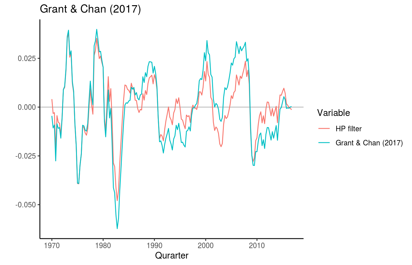

References

Balcilar, M. (2018). mFilter: Miscellaneous Time Series Filters. R package version 0.1-4. https://CRAN.R-project.org/package=mFilter

Baxter, M., & King, R. O. (1999). Measuring Business Cycles: Approximate Band-Pass Filters for Economic Time Series. Review of Economics and Statistics, 81(4), 575–593.

Chan, J., Koop, G., Poirier, D. J., & Tobias J. L. (2019). Bayesian econometric methods (2nd ed.). Cambridge: Cambridge University Press.

Grant, A. L., & Chan, J. C. C. (2017). Reconciling output gaps: Unobserved components model and Hodrick-Prescott filter, Journal of Economic Dynamics and Control, 75, 114-121.

Hamilton, J. D. (2018), Why you should never use the Hodrick-Prescott filter. Review of Economics and Statistics, 100(5), 831-843. https://doi.org/10.1162/rest_a_00706

Kim, D. and Oh, H.-S. (2014). EMD: Empirical Mode Decomposition and Hilbert Spectral Analysis. R package version 1.5.7.

Kožić, I., & Sever, I. (2014). Measuring business cycles: Empirical Mode Decomposition of economic time series. Economics Letters, 123(3), 287–290. https://doi.org/10.1016/j.econlet.2014.03.009

McTaggart, R., Daroczi, G., & Leung, C. (2018). Quandl: API Wrapper for Quandl.com. R package version 2.9.1. https://CRAN.R-project.org/package=Quandl

Shea, J. M. (2018). neverhpfilter: A Better Alternative to the Hodrick-Prescott Filter. R package version 0.2-0. https://CRAN.R-project.org/package=neverhpfilter

Stock, J. H., & Watson, M. W. (1999). Business Cycle Fluctuations in US Macroeconomic Time Series. In J. B. Taylor & M. Woodford (Eds.), Handbook of Macroeconomics. Handbook of Macroeconomics (pp. 3–64). Elsevier.

Whitcher, B. (2015). waveslim: Basic wavelet routines for one-, two- and three-dimensional signal processing. R package version 1.7.5. https://CRAN.R-project.org/package=waveslim

Wickham, H. (2016). ggplot2: Elegant Graphics for Data Analysis. Springer-Verlag New York.

Wickham, H., François, R., Henry, L., & Müller, K. (2018). dplyr: A Grammar of Data Manipulation. R package version 0.7.8. https://CRAN.R-project.org/package=dplyr

Yogo, M. (2008). Measuring business cycles: A wavelet analysis of economic time series. Economics Letters, 100(2), 208–212. https://doi.org/10.1016/j.econlet.2008.01.008