An Introduction to Impulse Response Analysis of VAR Models

Model and Data

To illustrate the concept of impulse response functions, examples from Lütkepohl (2007) are used. The required dataset can be downloaded from the textbook’s website. It contains quarterly, seasonally adjusted time series for West German fixed investment, disposable income, and consumption expenditures in billions of DM from 1960Q1 to 1982Q4.

# Download data
data <- read.table("http://www.jmulti.de/download/datasets/e1.dat", skip = 6, header = TRUE)

# Only use the first 76 observations so that there are 73 observations
# left for the estimated VAR(2) model after taking first differences.
data <- data[1:76, ]

# Convert to time series object
data <- ts(data, start = c(1960, 1), frequency = 4)

# Take logs and differences
data <- diff(log(data))

# Plot data
plot(data,  main = "Dataset E1 from Lütkepohl (2007)")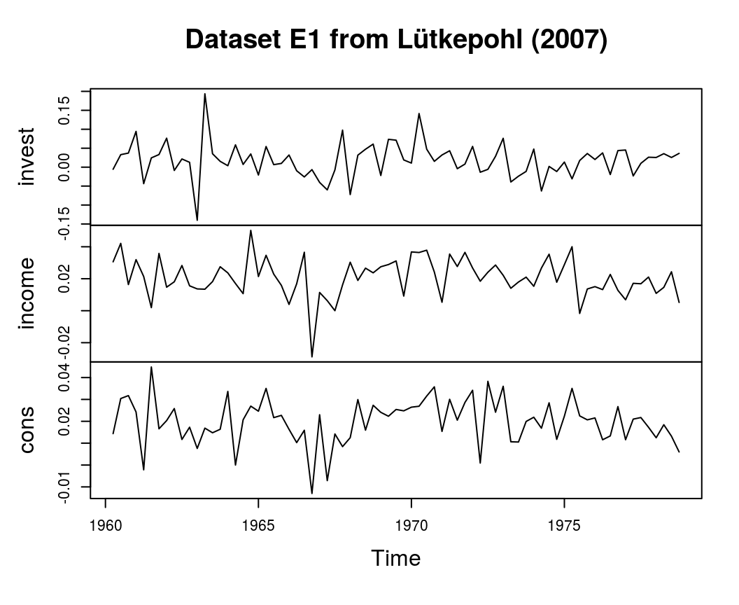

This data is used to estimate a VAR(2) model with a constant term:

\[ y_t = v + \sum_{i = 1}^{2} A_i y_{t-i} + u_t,\] where \(u_t \sim N(0, \Sigma)\).

Estimation

The VAR model can be estimated using the vars package of Pfaff (2008):

# Load package
library(vars)

# Estimate model
model <- VAR(data, p = 2, type = "const")

# Look at summary statistics
summary(model)

The results of the code should be identical to the results in section 3.2.3 of Lütkepohl (2007).

Forecast error impulse response

Since all variables in a VAR model depend on each other, individual coefficient estimates only provide limited information on the reaction of the system to a shock. In order to get a better picture of the model’s dynamic behaviour, impulse responses (IR) are used. The departure point of every impluse reponse function for a linear VAR model is its moving average (MA) representation, which is also the forecast error impulse response (FEIR) function. Mathematically, the FEIR \(\Phi_i\) for the \(i\)th period after the shock is obtained by \[\Phi_i = \sum_{j = 1}^{i} \Phi_{i - j} A_j, \ \ i = 1, 2, ...\] with \(\Phi_0 = I_{K}\) and \(A_j = 0 \text{ for } j>p\), where \(K\) is the number of endogenous variables and \(p\) is the lag order of the VAR model.

In R the irf function of the vars package can be used to obtain forecast error impulse responses. The following code calculates and plots the estimated response of consumption to a forecast error impulse in income with bootstrapped error bands¹:

feir <- irf(model, impulse = "income", response = "cons",
             n.ahead = 8, ortho = FALSE, runs = 1000)

plot(feir)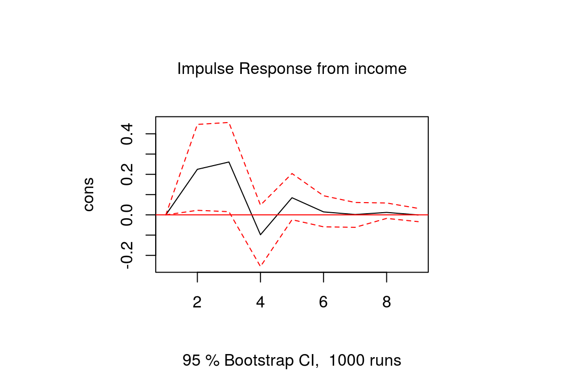

The identification problem

A caveat of FEIRs is that they cannot be used to assess contemporaneous reactions of variables. This can be seen in the previous plot, where the FEIR is zero in the first period. Mathematically, this can be explained by the fact that for the construction of \(\Phi_i\) only the coefficient matrices \(A_j\) are used, which contain no information on contemporaneous relationships. Information no the latter is rather contained in the off-diagonal elements of the symmetric variance-covariance matrix \(\Sigma\). For the used dataset it is estimated to be

# Calculate summary statistics
model_summary <- summary(model)

# Obtain variance-covariance matrix
model_summary$covres

##              invest       income         cons
## invest 2.129629e-03 7.161667e-05 1.232404e-04
## income 7.161667e-05 1.373377e-04 6.145867e-05
## cons   1.232404e-04 6.145867e-05 8.920351e-05

Since the off-diagonal elements of the estimated variance-covariance matrix are not zero, we can assume that there is contemporaneous correlation between the variables in the VAR model. This is confirmed by the correlation matrix, which corresponds to \(\Sigma\):

model_summary$corres

##           invest    income      cons
## invest 1.0000000 0.1324242 0.2827548
## income 0.1324242 1.0000000 0.5552611
## cons   0.2827548 0.5552611 1.0000000

However, those matrices only describe the correlation between the errors, but it remains unclear in which direction the causalities go. Identifying these causal relationships is one of the main challenges of any VAR analysis.

Regardless of the specific methods used to identify the shocks of a linear VAR model, further information on contemporaneous relationships can be introduced to the FEIR by simply multiplying it by a matrix \(F\):

\[\Theta_i = \Phi_i F\] for \(i = 0, 1, ...\). In the following some methodes to find \(F\) and their corresponding impulse responses are presented.

Orthogonal impulse responses

A common approach to identify the shocks of a VAR model is to use orthogonal impulse respones (OIR). The basic idea is to decompose the variance-covariance matrix so that \(\Sigma = PP^{\prime}\), where \(P\) is a lower triangular matrix with positve diagonal elements, which is often obtained by a Choleski decomposition. Given the estimated variance-covariance matrix \(P\) the decomposition can be obtained by

t(chol(model_summary$covres))

##             invest      income        cons
## invest 0.046147903 0.000000000 0.000000000
## income 0.001551894 0.011615909 0.000000000
## cons   0.002670552 0.004934117 0.007597773

From this matrix it can be seen that a shock to income has a contemporaneous effect on consumption, but not vice versa. The corresponding orthongonal impulse response function is then

\[\Theta^o_i = \Phi_i P.\]

In R the irf function of the vars package can be used to optain OIRs by setting the argument ortho = TRUE:

oir <- irf(model, impulse = "income", response = "cons",
           n.ahead = 8, ortho = TRUE, runs = 1000, seed = 12345)

plot(oir)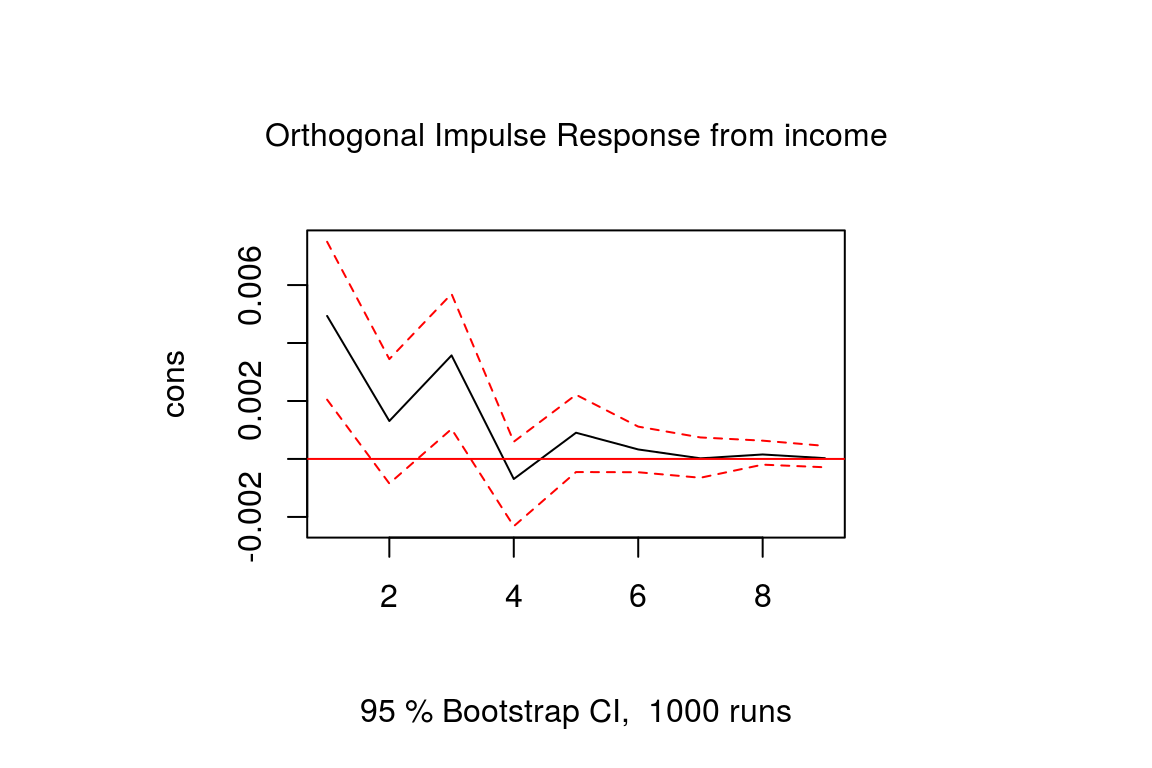

Note that the output of the Choleski decomposition is a lower triangular matrix so that the variable in the first row will never be sensitive to a contemporaneous shock of any other variable and the last variable in the system will be sensitive to shocks of all other variables. Therefore, the results of an OIR might be sensitive to the order of the variables and it is advised to estimate the above VAR model with different orders to see how strongly the resulting OIRs are affected by that.

Strucual impulse responses

Structural impulse responses (SIR) already take the identification problem into account during the estimation of the VAR model. For the structrual vector autoregressive (SVAR) model

\[ A_0 y_t = v + \sum_{i = 1}^{2} A_i y_{t-i} + \epsilon_t,\] where \(\epsilon_t \sim N(0, \Omega)\) with \(\Omega\) as a diagonal matrix of variances and \(A_0\) as lower triangular matrix with ones on its main diagonal the structural impulse response function becomes

\[\Theta^s_i = \Phi_i A_0^{-1}\]

Generalised impulse responses

Both orthogonal and structural impulse responses are constrained either by finding the right order of variables or by the identification of the estimated structural parameters. Koop et al. (1996) and Koop et al. (1998) propose a different kind of impulse response function, so-called generalised impulse responses (GIR). They are independent of the variable order, because they integrate the effects of other shocks out of the response. Mathematically, this is achieved in the following way:

\[\Theta^g_i = \Phi_i \sigma_{jj}^{-\frac{1}{2}} \Sigma,\] where \(\sigma_{jj}\) is the variance of the \(j\)th variable.

GIRs are very useful in the case of large systems, where structual relationships are hard to identify. They cannot really be interpreted as structural impulse responses, but they provide an accurate depiction of the historic development of the variable.

References

Koop, G., Pesaran, M. H., Potter, S. M. (1996). Impulse response analysis in nonlinear multivariate models. Journal of Econometrics 74, 119-147. doi:10.1016/0304-4076(95)01753-4

Lütkepohl, H. (2007). New introduction to multiple time series analysis (2nd ed.). Berlin: Springer.

Pesaran, H. H., Shin, Y. (1998). Generalized impulse response analysis in linear multivariate models. Economics Letters 58(1), 17-29. doi:10.1016/S0165-1765(97)00214-0

Pfaff, B. (2008). VAR, SVAR and SVEC Models: Implementation Within R Package vars. Journal of Statistical Software 27(4).