Stochastic Search Variable Selection
with tags r bvar var ssvs bvartools -Introduction
A general drawback of vector autoregressive (VAR) models is that the number of estimated coefficients increases disproportionately with the number of lags. Therefore, fewer information per parameter is available for the estimation as the number of lags increases. In the Bayesian VAR literature one approach to mitigate this so-called curse of dimensionality is stochastic search variable selection (SSVS) as proposed by George et al. (2008). The basic idea of SSVS is to assign commonly used prior variances to parameters, which should be included in a model, and prior variances close to zero to irrelevant parameters. By that, relevant parameters are estimated in the usual way and posterior draws of irrelevant variables are close to zero so that they have no significant effect on forecasts and impulse responses. This is achieved by adding a hierarchial prior to the model, where the relevance of a variable is assessed in each step of the sampling algorithm.1
This post presents code for the estimation of a Bayesian vector autoregressive (BVAR) model with SSVS. It uses dataset E1 from Lütkepohl (2007), which contains data on West German fixed investment, disposable income and consumption expenditures in billions of DM from 1960Q1 to 1982Q4. Following a related example in Lütkepohl (2007, Section 5.2.10) only the first 71 observations of a VAR(4) model are used. The bvartools package can be used to load the data and generate the data matrices:
library(bvartools) # install.packages("bvartools")

# Load and transform data
data("e1")
e1 <- diff(log(e1))

# Generate VAR
data <- gen_var(e1, p = 4, deterministic = "const")

# Get data matrices
y <- data$Y[, 1:71]
x <- data$Z[, 1:71]
Estimation
The prior variances of the parameters are set in accordance with the semiautomatic approach described in George et al. (2008). Hence, the prior variance of the \(i\)th parameter is set to \(\tau_{1,i}^2 = (10 \hat{\sigma}_i)^2\) if this parameter should be included in the model and to \(\tau_{0,i}^2 = (0.1 \hat{\sigma}_i)^2\) if it should be excluded. \(\hat{\sigma}_i\) is the standard error associated with the unconstrained least squares estimate of parameter \(i\). For all variables the prior inclusion probabilities are set to 0.5. The prior of the error variance-covariance matrix is uninformative.
# Reset random number generator for reproducibility
set.seed(1234567)

t <- ncol(y) # Number of observations
k <- nrow(y) # Number of endogenous variables
m <- k * nrow(x) # Number of estimated coefficients

# Coefficient priors
a_mu_prior <- matrix(0, m) # Vector of prior means

# SSVS priors (semiautomatic approach)
ols <- tcrossprod(y, x) %*% solve(tcrossprod(x)) # OLS estimates
sigma_ols <- tcrossprod(y - ols %*% x) / (t - nrow(x)) # OLS error covariance matrix
cov_ols <- kronecker(solve(tcrossprod(x)), sigma_ols)
se_ols <- matrix(sqrt(diag(cov_ols))) # OLS standard errors

tau0 <- se_ols * 0.1 # Prior if excluded
tau1 <- se_ols * 10 # Prior if included

# Prior for inclusion parameter
prob_prior <- matrix(0.5, m)

# Prior for variance-covariance matrix
u_sigma_df_prior <- 0 # Prior degrees of freedom
u_sigma_scale_prior <- diag(0, k) # Prior covariance matrix
u_sigma_df_post <- t + u_sigma_df_prior # Posterior degrees of freedom
The initial parameter values are set to zero and their corresponding prior variances are set to \(\tau_1^2\), which implies that all parameters should be estimated relatively freely in the first step of the Gibbs sampler.
# Initial values
a <- matrix(0, m)
a_v_i_prior <- diag(1 / c(tau1)^2, m) # Inverse of the prior covariance matrix

# Data containers for posterior draws
iter <- 15000 # Number of total Gibs sampler draws
burnin <- 5000 # Number of burn-in draws

store <- iter - burnin
draws_a <- matrix(NA, m, store)
draws_lambda <- matrix(NA, m, store)
draws_sigma <- matrix(NA, k^2, store)
SSVS can be added to a standard Gibbs sampler algorithm for VAR models in a straightforward manner. The ssvs function can be used to obtain a draw of inclusion parameters and its corresponding inverted prior variance matrix. It requires the current draw of parameters, standard errors \(\tau_0\) and \(\tau_1\), and prior inclusion probabilities as arguments. In this example constant terms are excluded from SSVS, which is achieved by specifying include = 1:36. Hence, only parameters 1 to 36 are considered by the function and the remaining three parameters have prior variances that correspond to their values in \(\tau_1^2\).
# Reset random number generator for reproducibility
set.seed(1234567)

# Start Gibbs sampler
for (draw in 1:iter) {
  # Draw variance-covariance matrix
  u <- y - matrix(a, k) %*% x # Obtain residuals
  # Scale posterior
  u_sigma_scale_post <- solve(u_sigma_scale_prior + tcrossprod(u))
  # Draw posterior of inverse sigma
  u_sigma_i <- matrix(rWishart(1, u_sigma_df_post, u_sigma_scale_post)[,, 1], k)
  # Obtain sigma
  u_sigma <- solve(u_sigma_i)

  # Draw conditional mean parameters
  a <- post_normal(y, x, u_sigma_i, a_mu_prior, a_v_i_prior)

  # Draw inclusion parameters and update priors
  temp <- ssvs(a, tau0, tau1, prob_prior, include = 1:36)
  a_v_i_prior <- temp$V_i # Update prior

  # Store draws
  if (draw > burnin) {
    draws_a[, draw - burnin] <- a
    draws_lambda[, draw - burnin] <- temp$lambda
    draws_sigma[, draw - burnin] <- u_sigma
  }
}
The output of a Gibbs sampler with SSVS can be further analysed in the usual way. Therefore, point estimates can be obtained by calculating the means of the parameters’ posterior draws:
A <- rowMeans(draws_a) # Obtain means for every parameter
A <- matrix(A, k) # Transform mean vector into matrix
A <- round(A, 3) # Round values
dimnames(A) <- list(dimnames(y)[[1]], dimnames(x)[[1]]) # Rename matrix dimensions

t(A) # Print
## invest income cons
## invest.1 -0.102 0.011 -0.002
## income.1 0.044 -0.031 0.168
## cons.1 0.074 0.140 -0.287
## invest.2 -0.013 0.002 0.004
## income.2 0.015 0.004 0.315
## cons.2 0.027 -0.001 0.006
## invest.3 0.033 0.000 0.000
## income.3 -0.008 0.021 0.013
## cons.3 -0.043 0.007 0.019
## invest.4 0.250 0.001 -0.005
## income.4 -0.064 -0.010 0.025
## cons.4 -0.023 0.001 0.000
## const 0.014 0.017 0.014It is also possible to obtain the posterior inclusion probabilites of each variable by calculating the means of their posterior draws. As can be seen in the output below, only few variables appear to be relevant in the VAR(4) model, because most inclusion probabilities are relatively low. The inclusion probabilities of the constant terms are 100 percent, because they were excluded from SSVS.
lambda <- rowMeans(draws_lambda) # Obtain means for every row
lambda <- matrix(lambda, k) # Transform mean vector into a matrix
lambda <- round(lambda, 2) # Round values
dimnames(lambda) <- list(dimnames(y)[[1]], dimnames(x)[[1]]) # Rename matrix dimensions

t(lambda) # Print
## invest income cons
## invest.1 0.43 0.23 0.10
## income.1 0.10 0.18 0.67
## cons.1 0.11 0.40 0.77
## invest.2 0.11 0.09 0.14
## income.2 0.08 0.07 0.98
## cons.2 0.07 0.06 0.08
## invest.3 0.19 0.07 0.06
## income.3 0.06 0.13 0.10
## cons.3 0.09 0.07 0.12
## invest.4 0.78 0.09 0.16
## income.4 0.13 0.09 0.18
## cons.4 0.09 0.07 0.06
## const 1.00 1.00 1.00Given these values, the researcher could proceed in the usual way and obtain forecasts and impulse responses based on the output of the Gibbs sampler. The advantage of this approach is that it does not only take into account parameter uncertainty, but also model uncertainty. This can be illustrated by the histogram of the posterior draws of the 6th coefficient, which describes the relationship between the first lag of income and the current value of consumption.
hist(draws_a[6,], main = "Consumption ~ First lag of income", xlab = "Value of posterior draw")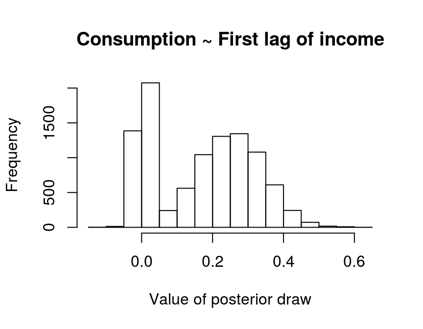
A non-negligible mass of some 23 percent, i.e. 1 - 0.67, of the parameter draws is concentrated around zero. This is the result of SSVS, where posterior draws are close to zero if a constant is assessed to be irrelevant during an iteration of the Gibbs sampler and, therefore, \(\tau_{0,6}^2\) is used as its prior variance. On the other hand, about 67 percent of the draws are dispersed around a positive value, where SSVS suggests to include the variable in the model and the larger value \(\tau_{1,6}^2\) is used as prior variance. Model uncertainty is then described by the two peaks and parameter uncertainty by the dispersion of the posterior draws around them.
However, if the researcher prefers not want to work with a model, where the relevance of a variable can change from one step of the sampling algorithm to another, a different approach would be to work only with a highly probable model. This can be done with a further simulation, where very tight priors are used for irrelevant variables and relatively uninformative priors for relevant parameters. In this example, coefficients with a posterior inclusion probability of above 40 percent are considered to be relevant.2 The prior variance is set to 0.00001 for irrelevant and to 9 for relevant variables. No additional SSVS step is required. Everything else remains unchanged.
# Select variables that should be included
include_var <- c(lambda >= .4)

# Update prior variances
diag(a_v_i_prior)[!include_var] <- 100000 # Very tight prior close to zero
diag(a_v_i_prior)[include_var] <- 1 / 9 # Relatively uninformative prior

# Data containers for posterior draws
draws_a <- matrix(NA, m, store)
draws_sigma <- matrix(NA, k^2, store)

# Start Gibbs sampler
for (draw in 1:iter) {
  # Draw conditional mean parameters
  a <- post_normal(y, x, u_sigma_i, a_mu_prior, a_v_i_prior)

  # Draw variance-covariance matrix
  u <- y - matrix(a, k) %*% x # Obtain residuals
  u_sigma_scale_post <- solve(u_sigma_scale_prior + tcrossprod(u))
  u_sigma_i <- matrix(rWishart(1, u_sigma_df_post, u_sigma_scale_post)[,, 1], k)
  u_sigma <- solve(u_sigma_i) # Invert Sigma_i to obtain Sigma

  # Store draws
  if (draw > burnin) {
    draws_a[, draw - burnin] <- a
    draws_sigma[, draw - burnin] <- u_sigma
  }
}
The means of the posterior draws are similar to the OLS estimates in Lütkepohl (2007, Section 5.2.10):
A <- rowMeans(draws_a) # Obtain means for every row
A <- matrix(A, k) # Transform mean vector into a matrix
A <- round(A, 3) # Round values
dimnames(A) <- list(dimnames(y)[[1]], dimnames(x)[[1]]) # Rename matrix dimensions

t(A) # Print
## invest income cons
## invest.1 -0.219 0.001 -0.001
## income.1 0.000 0.000 0.262
## cons.1 0.000 0.238 -0.334
## invest.2 0.000 0.000 0.001
## income.2 0.000 0.000 0.329
## cons.2 0.000 0.000 0.000
## invest.3 0.000 0.000 0.000
## income.3 0.000 0.000 0.000
## cons.3 0.000 0.000 0.000
## invest.4 0.328 0.000 -0.001
## income.4 0.000 0.000 0.000
## cons.4 0.000 0.000 0.000
## const 0.015 0.015 0.014Evaluation
The bvar function can be used to collect relevant output of the Gibbs sampler into a standardised object, which can be used by further functions such as predict to obtain forecasts or irf for impulse respons analysis.
bvar_est <- bvar(y = y, x = x, A = draws_a[1:36,],
                 C = draws_a[37:39, ], Sigma = draws_sigma)
Posterior draws can be thinned with function thin:
bvar_est <- thin(bvar_est, thin = 5)Forecasts
Forecasts with credible bands can be obtained with the function predict. If the model contains deterministic terms, new values can be provided in the argument new_D. If no values are provided, the function sets them to zero. The number of rows of new_D must be the same as the argument n.ahead.
bvar_pred <- predict(bvar_est, n.ahead = 10, new_D = rep(1, 10))

plot(bvar_pred)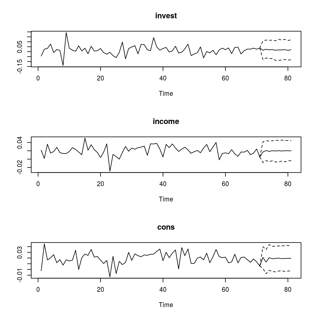
Impulse response analysis
OIR <- irf(bvar_est, impulse = "income", response = "cons", n.ahead = 8, type = "oir")

plot(OIR, main = "Orthogonalised Impulse Response", xlab = "Period", ylab = "Response")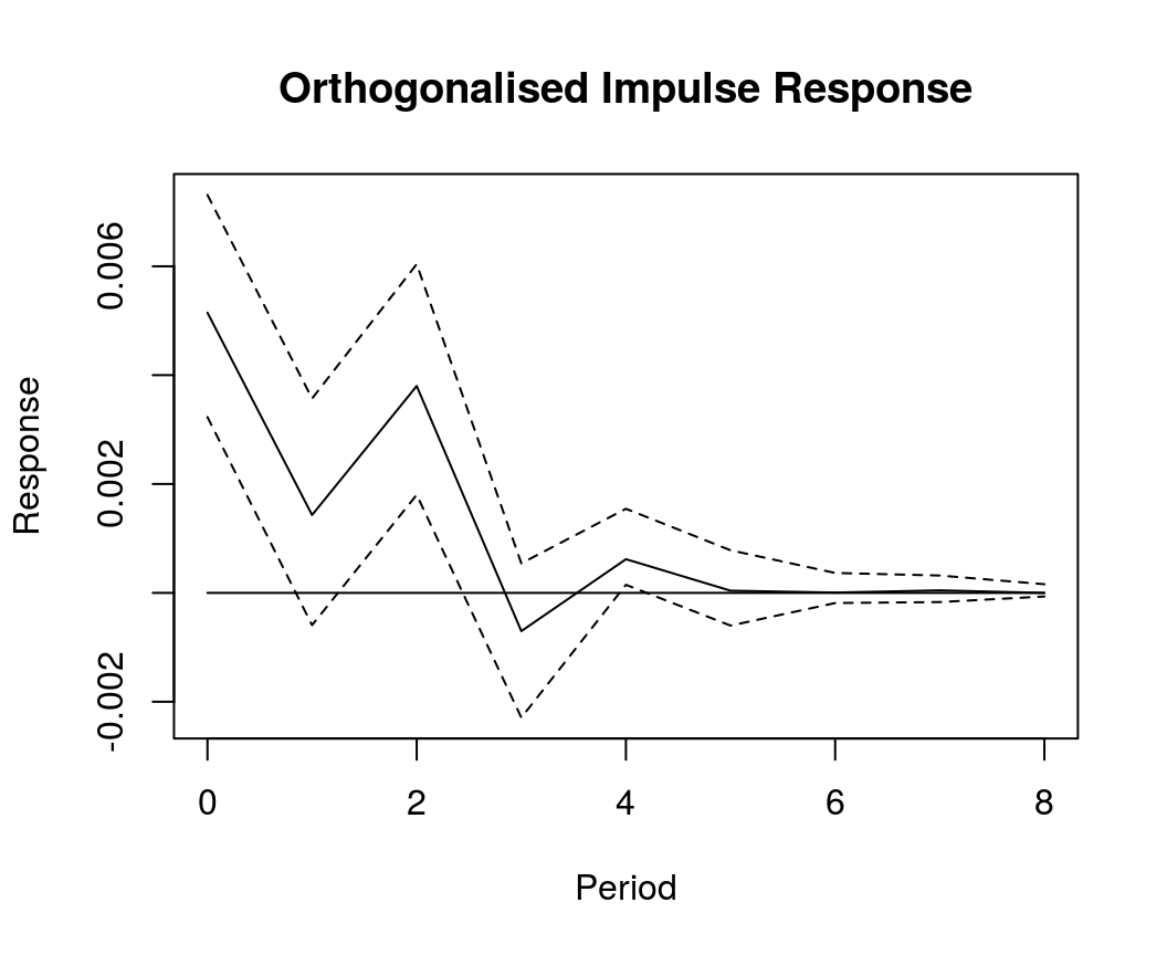
References
George, E. I., Sun, D., & Ni, S. (2008). Bayesian stochastic search for VAR model restrictions. Journal of Econometrics, 142(1), 553-580. https://doi.org/10.1016/j.jeconom.2007.08.017
Koop, G., & Korobilis, D. (2010). Bayesian multivariate time series methods for empirical macroeconomics. Foundations and trends in econometrics, 3(4), 267-358. https://dx.doi.org/10.1561/0800000013
Lütkepohl, H. (2007). New introduction to multiple time series analysis (2nd ed.). Berlin: Springer.