An Introduction to Structural Vector Autoregression (SVAR)
Posted in r var with tags r var svar vector autoregression -Vector autoregressive (VAR) models constitute a rather general approach to modelling multivariate time series. A critical drawback of those models in their standard form is their missing ability to describe contemporaneous relationships between the analysed variables. This becomes a central issue in the impulse response analysis for such models, where it is important to know the contemporaneous effects of a shock to the economy. Usually, researchers address this by using orthogonal impulse responses, where the correlation between the errors is obtained from the (lower) Cholesky decomposition of the error covariance matrix. This requires them to arrange the variables of the model in a suitable order. An alternative to this approach is to use so-called structural vector autoregressive (SVAR) models, where the relationship between contemporaneous variables is modelled more directly. This post provides an introduction to the concept of SVAR models and how they can be estimated in R.
What does the term “structual” mean?
To understand what a structural VAR model is, let’s repeat the main characteristics of a standard reduced form VAR model:
yt=A1yt−1+ut with ut∼(0,Σ),
To understand SVAR models, it is important to look more closely at the variance-covariance matrix Σ. It contains the variances of the endogenous variable on its diagonal elements and covariances of the errors on the off-diagonal elements. The covariances contain information about contemporaneous effects each variable has on the others. The covariance matrices of standard VAR models is symmetric, i.e. the elements to the top-right of the diagonal (the “upper triangular”) mirror the elements to the bottom-left of the diagonal (the “lower triangular”). This reflects the idea that the relations between the endogenous variables only reflect correlations and do not allow to make statements about causal relationships.
Contemporaneous causality or, more precisely, the structural relationships between the variables is analysed in the context of SVAR models, which impose special restrictions on the covariance matrix and – depending on the model – on other coefficient matrices as well. The drawback of this approach is that it depends on the more or less subjective assumptions made by the researcher. For many researchers this is too much subjectiv information, even if sound economic theory is used to justify them. However, they can be useful tools and that is why it is worth to look into them.
Lütkepohl (2007) mentions four approaches to model structural relationships between the endogenouse variables of a VAR model: The A-model, the B-model, the AB-model and long-run restrictions à la Blanchard and Quah (1989).
The A-model
The A-model assumes that the covariance matrix is diagonal - i.e. it only contains the variances of the error term - and contemporaneous relationships between the observable variables are described by an additional matrix A so that
Ayt=A∗1yt−1+...+A∗pyt−p+ϵt,
Matrix A has the special form:
A=[10⋯0a2110⋮⋱⋮aK1aK2⋯1]
Beside the normalisation that is achieved by setting the diagonal elements of A to one, the matrix contains (K(K−1)/2 further restrictions, which are needed to obtain unique estimates of the structural coefficients. If less restirctions were provided, there would be mathematical problems - to express it in a simple way. In the above example, the upper triangular elements of the matrix are set to zero and the elements below the diagonal are freely estimated. However, it would also be possible to estimate a coefficient in the upper triangular area, if a value in the lower triangular area were set to zero. Furthermore, it would be possible to set more than (K(K−1)/2 elements of A to zero. In this case the model is said to be over-identified.
The B-model
The B-model describes the structural relationships of the errors directly by adding a matrix B to the error term and normalises the error variances to unity so that
yt=A1yt−1+...+Apyt−p+Bϵt,
The AB-model
The AB-model is a mixture of the A- and B-model, where the errors of the VAR are modelled as
Aut=Bϵt with ϵt∼(0,IK).
This general form would require to specify more restrictions than in the A- or B-model. Thus, one of the matrices is usually replaced by an identiy matrix and the other contains the necessary restrictions. This model can be useful to estimate, for example, a system of equations, which describe the IS-LM-model.
Long-run restirctions à la Blanchard-Quah
Blanchard and Quah (1989) propose an approach, which does not require to directly impose restrictions on the structural matrices A or B. Instead, structural innovations can be identified by looking at the accumulated effects of shocks and placing zero restrictions on those accumulated relationships, which die out and become zero in the long run.
Estimation
Data
For this illustration we generate an artificial data set with three endogenous variables, which followe the data generating process
yt=A1yt−1+Bϵt,
where
A1=[0.30.120.6900.30.480.240.240.3], B=[100−0.1410−0.060.391] and ϵt∼N(0,I3).
# Reset random number generator for reproducibility
set.seed(24579)

tt <- 500 # Number of time series observations

# Coefficient matrix
A_1 <- matrix(c(0.3, 0, 0.24,
                0.12, 0.3, 0.24,
                0.69, 0.48, 0.3), 3)

# Structural coefficients
B <- diag(1, 3)
B[lower.tri(B)] <- c(-0.14, -0.06, 0.39)

# Generate series
series <- matrix(rnorm(3, 0, 1), 3, tt + 1) # Raw series with zeros
for (i in 2:(tt + 1)){
  series[, i] <- A_1 %*% series[, i - 1] +  B %*% rnorm(3, 0, 1)
}

series <- ts(t(series)) # Convert to time series object
dimnames(series)[[2]] <- c("S1", "S2", "S3") # Rename variables

# Plot the series
plot.ts(series, main = "Artificial time series")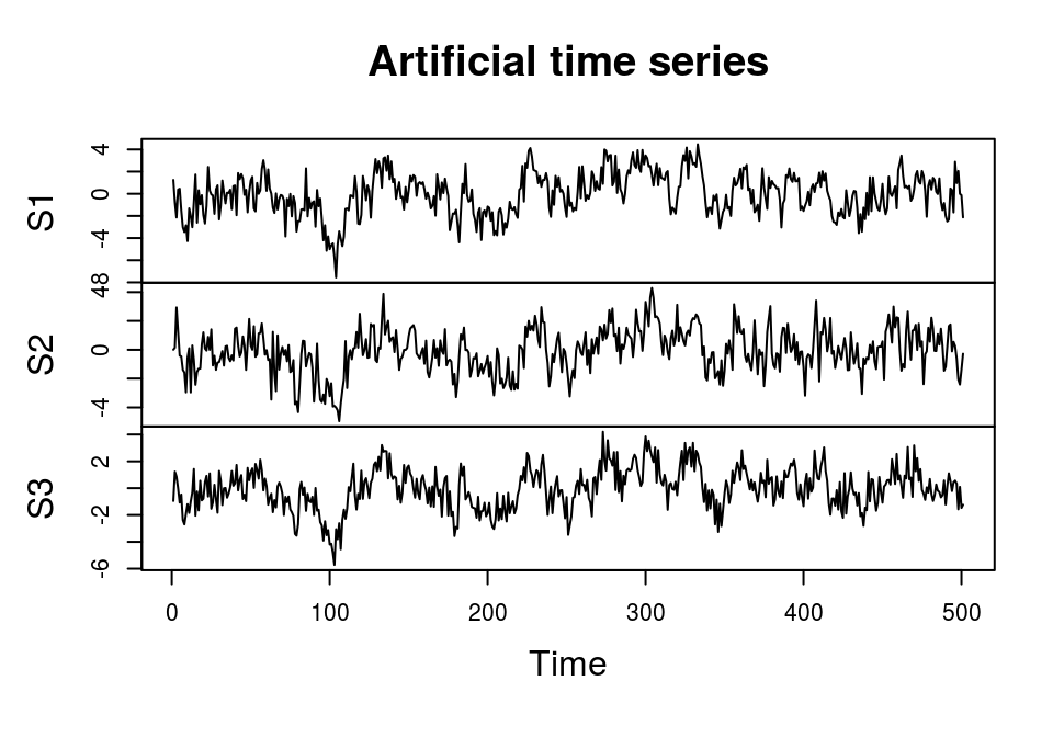
The vars package (Pfaff, 2008) provides functions to estimate structural VARs in R. The workflow is divided into two steps, where the first consists in estimating a standard VAR model using the VAR function:
library(vars)

# Estimate reduced form VAR
var_est <- VAR(series, p = 1, type = "none")

var_est
##
## VAR Estimation Results:
## =======================
##
## Estimated coefficients for equation S1:
## =======================================
## Call:
## S1 = S1.l1 + S2.l1 + S3.l1
##
## S1.l1 S2.l1 S3.l1
## 0.3288079 0.1124078 0.6809865
##
##
## Estimated coefficients for equation S2:
## =======================================
## Call:
## S2 = S1.l1 + S2.l1 + S3.l1
##
## S1.l1 S2.l1 S3.l1
## -0.001530688 0.289578440 0.512701274
##
##
## Estimated coefficients for equation S3:
## =======================================
## Call:
## S3 = S1.l1 + S2.l1 + S3.l1
##
## S1.l1 S2.l1 S3.l1
## 0.2401861 0.2519319 0.3186145The estimated coefficients are reasonably close to the true coefficients. In the next step the resulting object is used in function SVAR to estimate the various structural models.
A-model
The A-model requires to specify a matrix Amat, which contains the K(K−1)/2 restrictions. In the following example, we create a diagonal matrix with ones as diagonal elements and zeros in its upper triangle. The lower triangular elements are set to NA, which indicates that they should be estimated.
# Estimate structural coefficients
a <- diag(1, 3)
a[lower.tri(a)] <- NA

svar_est_a <- SVAR(var_est, Amat = a, max.iter = 1000)

svar_est_a
##
## SVAR Estimation Results:
## ========================
##
##
## Estimated A matrix:
## S1 S2 S3
## S1 1.00000 0.0000 0
## S2 0.18177 1.0000 0
## S3 0.05078 -0.3132 1The result is not equal to matrix B, because we estimated an A-model. In order to translate it into the structural coefficients of the B-model, we only have to obtain the inverse of the matrix:
solve(svar_est_a$A)## S1 S2 S3
## S1 1.0000000 0.0000000 0
## S2 -0.1817747 1.0000000 0
## S3 -0.1077103 0.3131988 1Confidence intervals for the structural coefficients can be obtained by directly accessing the respective element in svar_est_a:
svar_est_a$Ase## S1 S2 S3
## S1 0.00000000 0.00000000 0
## S2 0.04472136 0.00000000 0
## S3 0.04545420 0.04472136 0B-model
B-modes are estimated in a similar way as A-models by specifying a matrix Bmat, which contains restrictions on the structural matrix B. In the following example B is equal to Amat above.
# Create structural matrix with restrictions
b <- diag(1, 3)
b[lower.tri(b)] <- NA

# Estimate
svar_est_b <- SVAR(var_est, Bmat = b)

# Show result
svar_est_b
##
## SVAR Estimation Results:
## ========================
##
##
## Estimated B matrix:
## S1 S2 S3
## S1 1.0000 0.0000 0
## S2 -0.1818 1.0000 0
## S3 -0.1077 0.3132 1Again, confidence intervals of the structural coefficients can be obtained by directly accessing the respective element in svar_est_b:
svar_est_b$Bse## S1 S2 S3
## S1 0.00000000 0.00000000 0
## S2 0.04472136 0.00000000 0
## S3 0.04686349 0.04472136 0Literature
Blanchard, O., & Quah, D. (1989). The dynamic effects of aggregate demand and supply disturbances. American Economic Review 79, 655-673.
Lütkepohl, H. (2007). New Introduction to Multiple Time Series Analyis (2nd ed.). Berlin: Springer.
Bernhard Pfaff (2008). VAR, SVAR and SVEC Models: Implementation Within R Package vars. Journal of Statistical Software 27(4).
Sims, C. (1980). Macroeconomics and Reality. Econometrica, 48(1), 1-48.