An Introduction to Vector Error Correction Models (VECMs)
with tags r vec cointegration vars urca tsDyn -One of the prerequisits for the estimation of a vector autoregressive (VAR) model is that the analysed time series are stationary. However, economic theory suggests that there exist equilibrium relations between economic variables in their levels, which can render these variables stationary without taking differences. This is called cointegration. Since knowing the size of such relationships can improve the results of an analysis, it would be desireable to have an econometric model, which is able to capture them. So-called vector error correction models (VECMs) belong to this class of models. The following text presents the basic concept of VECMs and guides through the estimation of such a model in R.
Model and data
Vector error correction models are very similar to VAR models and can have the following form:
\[\Delta x_t = \Pi x_{t-1} + \sum_{l = 1}^{p-1} \Gamma_l \Delta x_{t-l} + C d_t + \epsilon_t,\] where \(\Delta x\) is the first difference of the variables in vector \(x\), \(Pi\) is a coefficient matrix of cointegrating relationships, \(\Gamma\) is a coefficient matrix of the lags of differenced variables of \(x\), \(d\) is a vector of deterministic terms and \(C\) its corresponding coefficient matrix. \(p\) is the lag order of the model in its VAR form and \(\epsilon\) is an error term with zero mean and variance-covariance matrix \(\Sigma\).
The above equation shows that the only difference to a VAR model is the error correction term \(\Pi x_{t-1}\), which captures the effect of how the growth rate of a variable in \(x\) changes, if one of the variables departs from its equilibrium value. The coefficient matrix \(\Pi\) can be written as the matrix product \(\Pi = \alpha \beta^{\prime}\) so that the error correction term becomes \(\alpha \beta^{\prime} x_{t-1}\). The cointegration matrix \(\beta\) contains information on the equilibrium relationships between the variables in levels. The vector described by \(\beta^{\prime} x_{t-1}\) can be interpreted as the distance of the variables form their equilibrium values. \(\alpha\) is a so-called loading matrix describing the speed at which a dependent variable converges back to its equilibrium value.
Note that \(\Pi\) is assumed to be of reduced rank, which means that \(\alpha\) is a \(K \times r\) matrix and \(\beta\) is a \(K^{co} \times r\) matrix, where \(K\) is the number of endogenous variables, \(K^{co}\) is the number of variables in the cointegration term and \(r\) is the rank of \(\Pi\), which describes the number of cointegrating relationships that exist between the variables. Note that if \(r = 0\), there is no cointegration between the variables so that \(\Pi = 0\).
To illustrate the estimation of VECMs in R, we use dataset E6 from Lütkepohl (2007), which contains quarterly, seasonally unadjusted time series for German long-term interest and inflation rates from 1972Q2 to 1998Q4. It comes with the bvartools package.
library(bvartools) # Load the package, which contains the data
data("e6") # Load data
plot(e6) # Plot data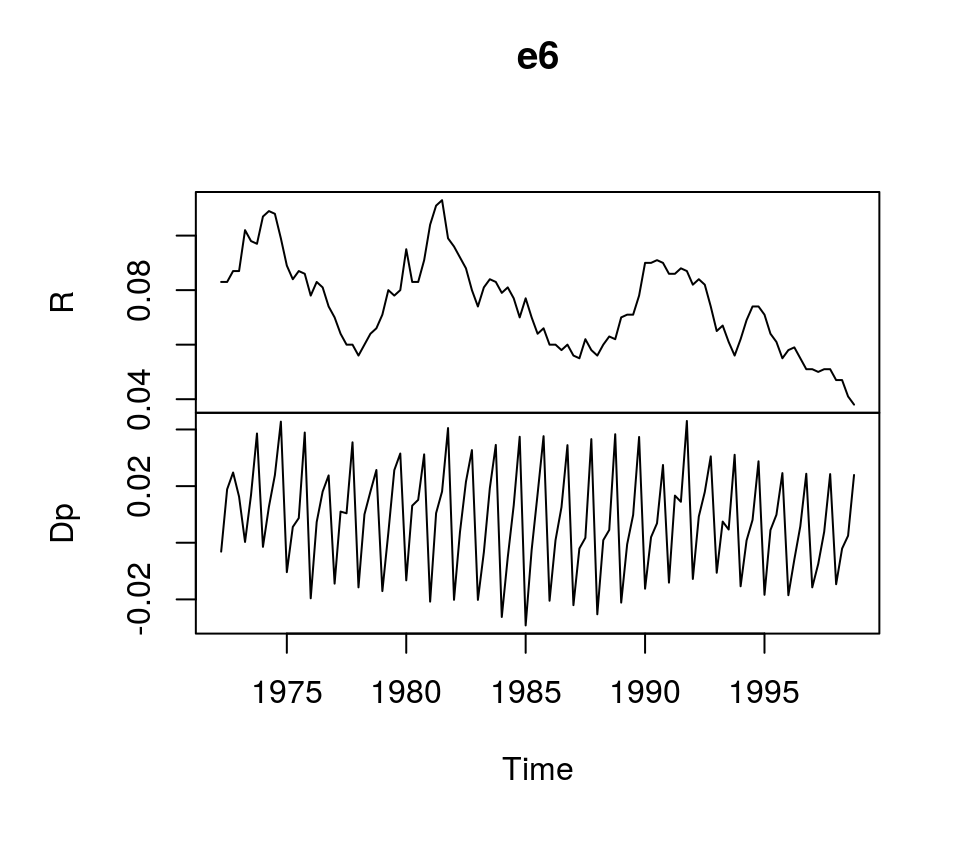
Estimation
There are multiple ways to estimate VEC models. A first approach would be to use ordinary least squares, which yields accurate result, but does not allow to estimate the cointegrating relations among the variables. The estimated generalised least squares (EGLS) approach would be an alternative. However, the most popular estimator for VECMs seems to be the maximum likelihood estimator of Johansen (1995), which is implemented in R by the ca.jo function of the urca package of Pfaff (2008a). Alternatively, function VECM of the tsDyn package of Di Narzo et al. (2020) can be used as well.1
But before the VEC model can be estimated, the lag order \(p\), the rank of the cointegration matrix \(r\) and deterministic terms have to be specified. A valid strategy to choose the lag order is to estimated the VAR in levels and choose the lag specification that minimises an Information criterion. Since the time series show strong seasonal pattern, we control for this by specifying season = 4, where 4 is the frequency of the data.
library(vars) # Load package

# Estimate VAR
var_aic <- VAR(e6, type = "const", lag.max = 8, ic = "AIC", season = 4)

# Lag order suggested by AIC
var_aic$p
## AIC(n)
## 4According to the AIC, a lag order of 4 can be used, which is the same value used in Lütkepohl (2007). This means the VEC model corresponding to the VAR in levels has 3 lags. Since the ca.jo function requires the lag order of the VAR model we set K = 4.2
The inclusion of deterministic terms in a VECM is a delicate issue. Without going into detail a common strategy is to add a linear trend to the error correction term and a constant to the non-cointegration part of the equation. For this example we follow Lütkepohl (2007) and add a constant term and seasonal dummies to the non-cointegration part of the equation.
The ca.jo function does not just estimate the VECM. It also calculates the test statistics for different specificaions of \(r\) and the user can choose between two alternative approaches, the trace and the eigenvalue test. For this example the trace test is used, i.e. type = "trace".
By default, the ca.jo function sets spec = "longrun" This specification would mean that the error correction term does not refer to the first lag of the variables in levels as decribed above, but to the \(p-1\)th lag instead. By setting spec = "transitory" the first lag will be used instead. Further information on the interpretation the two alternatives can be found in the function’s documentation ?ca.jo.
For further details on VEC modelling I recommend Lütkepohl (2006, Chapters 6, 7 and 8).
library(urca) # Load package

# Estimate
vec <- ca.jo(e6, ecdet = "none", type = "trace",
             K = 4, spec = "transitory", season = 4)

summary(vec)
##
## ######################
## # Johansen-Procedure #
## ######################
##
## Test type: trace statistic , with linear trend
##
## Eigenvalues (lambda):
## [1] 0.15184737 0.03652339
##
## Values of teststatistic and critical values of test:
##
## test 10pct 5pct 1pct
## r <= 1 | 3.83 6.50 8.18 11.65
## r = 0 | 20.80 15.66 17.95 23.52
##
## Eigenvectors, normalised to first column:
## (These are the cointegration relations)
##
## R.l1 Dp.l1
## R.l1 1.000000 1.000000
## Dp.l1 -3.961937 1.700513
##
## Weights W:
## (This is the loading matrix)
##
## R.l1 Dp.l1
## R.d -0.1028717 -0.03938511
## Dp.d 0.1577005 -0.02146119The trace test suggests that \(r=1\) and the first columns of the estimates of the cointegration relations \(\beta\) and the loading matrix \(\alpha\) correspond to the results of the ML estimator in Lütkepohl (2007, Ch. 7):
# Beta
round(vec@V, 2)
## R.l1 Dp.l1
## R.l1 1.00 1.0
## Dp.l1 -3.96 1.7# Alpha
round(vec@W, 2)## R.l1 Dp.l1
## R.d -0.10 -0.04
## Dp.d 0.16 -0.02However, the estimated coefficients of the non-cointegration part of the model correspond to the results of the EGLS estimator.
round(vec@GAMMA, 2)## constant sd1 sd2 sd3 R.dl1 Dp.dl1 R.dl2 Dp.dl2 R.dl3 Dp.dl3
## R.d 0.01 0.01 0.00 0.00 0.29 -0.16 0.01 -0.19 0.25 -0.09
## Dp.d -0.01 0.02 0.02 0.03 0.08 -0.31 0.01 -0.37 0.04 -0.34The deterministic terms are different from the results in Lütkepohl (2006), because different reference dates are used.
Using the the tsDyn package, estimates of the coefficients can be obtained in the following way:
# Load package
library(tsDyn)

# Obtain constant and seasonal dummies
seas <- gen_vec(data = e6, p = 4, r = 1, const = "unrestricted", seasonal = "unrestricted")
# Lag order p is 4 since gen_vec assumes that p corresponds to VAR form
seas <- seas$data$X[, 7:10]

# Estimate
est_tsdyn <- VECM(e6, lag = 3, r = 1, include = "none", estim = "ML", exogen = seas)

# Print results
summary(est_tsdyn)
## #############
## ###Model VECM
## #############
## Full sample size: 107 End sample size: 103
## Number of variables: 2 Number of estimated slope parameters 22
## AIC -2142.333 BIC -2081.734 SSR 0.005033587
## Cointegrating vector (estimated by ML):
## R Dp
## r1 1 -3.961937
##
##
## ECT R -1 Dp -1
## Equation R -0.1029(0.0471)* 0.2688(0.1062)* -0.2102(0.1581)
## Equation Dp 0.1577(0.0445)*** 0.0654(0.1003) -0.3392(0.1493)*
## R -2 Dp -2 R -3
## Equation R -0.0178(0.1069) -0.2230(0.1276). 0.2228(0.1032)*
## Equation Dp -0.0043(0.1010) -0.3908(0.1205)** 0.0184(0.0975)
## Dp -3 const season.1
## Equation R -0.1076(0.0855) 0.0015(0.0038) 0.0015(0.0051)
## Equation Dp -0.3472(0.0808)*** 0.0102(0.0036)** -0.0341(0.0048)***
## season.2 season.3
## Equation R 0.0089(0.0053). -0.0004(0.0051)
## Equation Dp -0.0179(0.0050)*** -0.0164(0.0048)***Impulse response analyis
The impulse response function of a VECM is usually obtained from its VAR form. The function vec2var of the vars package can be used to transform the output of the ca.jo function into an object that can be handled by the irf function of the vars package. Note that since ur.jo does not set the rank \(r\) of the cointegration matrix automatically, it has to be specified manually.
# Transform VEC to VAR with r = 1
var <- vec2var(vec, r = 1)
The impulse response function is then calculated in the usual manner by using the irf function.
# Obtain IRF
ir <- irf(var, n.ahead = 20, impulse = "R", response = "Dp",
          ortho = FALSE, runs = 500)

# Plot
plot(ir)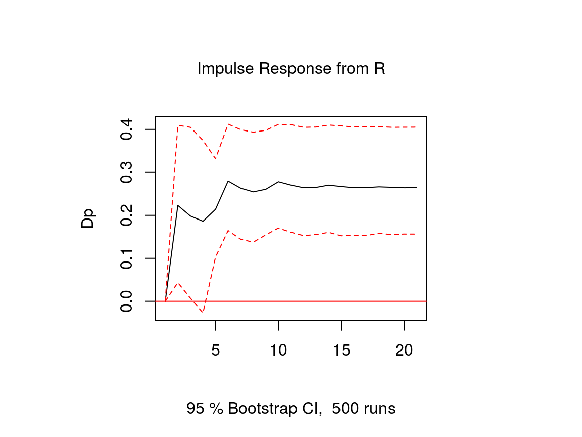
Note that an important difference to stationary VAR models is that the impulse response of a cointegrated VAR model does not neccessarily approach zero, because the variables are not stationary.
References
Lütkepohl, H. (2006). New introduction to multiple time series analysis (2nd ed.). Berlin: Springer.
Di Narzo, A. F., Aznarte, J. L., Stigler, M., &and Tsung-wu, H. (2020). tsDyn: Nonlinear Time Series Models with Regime Switching. R package version 10-1.2. https://CRAN.R-project.org/package=tsDyn
Pfaff, B. (2008a). Analysis of Integrated and Cointegrated Time Series with R. Second Edition. New York: Springer.
Pfaff, B. (2008b). VAR, SVAR and SVEC Models: Implementation Within R Package vars. Journal of Statistical Software 27(4).