Heteroskedasticity Robust Standard Errors in R

with tags heteroskedasticity t-test F-test robust-error - Franz X. Mohr, Created: December 24, 2018, Last update: December 24, 2018

Although heteroskedasticity does not produce biased OLS estimates, it leads to a bias in the variance-covariance matrix. This means that standard model testing methods such as t tests or F tests cannot be relied on any longer. This post provides an intuitive illustration of heteroskedasticity and covers the calculation of standard errors that are robust to it.

Data

A popular illustration of heteroskedasticity is the relationship between saving and income, which is shown in the following graph. The dataset is contained the wooldridge package.¹

# Load packages
library(dplyr)
library(ggplot2)
library(wooldridge)

# Load the sample
data("saving")

# Only use positive values of saving, which are smaller than income
saving <- saving %>%
  filter(sav > 0,
         inc < 20000,
         sav < inc)

# Plot
ggplot(saving, aes(x = inc, y = sav)) +
  geom_point() +
  geom_smooth(method = "lm", se = FALSE) +
  labs(x = "Annual income", y = "Annual savings")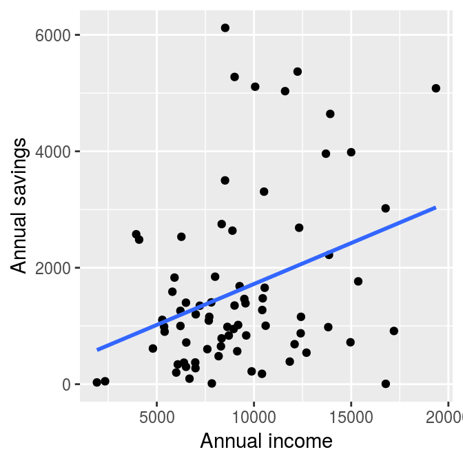

The regression line in the graph shows a clear positive relationship between saving and income. However, as income increases, the differences between the observations and the regression line become larger. This means that there is higher uncertainty about the estimated relationship between the two variables at higher income levels. This is an example of heteroskedasticity.

Since standard model testing methods rely on the assumption that there is no correlation between the independent variables and the variance of the dependent variable, the usual standard errors are not very reliable in the presence of heteroskedasticity. Fortunately, the calculation of robust standard errors can help to mitigate this problem.

Robust standard errors

The regression line above was derived from the model \[sav_i = \beta_0 + \beta_1 inc_i + \epsilon_i,\] for which the following code produces the standard R output:

# Estimate the model
model <- lm(sav ~ inc, data = saving)

# Print estimates and standard test statistics
summary(model)

## 
## Call:
## lm(formula = sav ~ inc, data = saving)
## 
## Residuals:
##     Min      1Q  Median      3Q     Max 
## -2667.8  -874.5  -302.7   431.1  4606.6 
## 
## Coefficients:
##              Estimate Std. Error t value Pr(>|t|)   
## (Intercept) 316.19835  462.06882   0.684  0.49595   
## inc           0.14052    0.04672   3.007  0.00361 **
## ---
## Signif. codes:  0 '***' 0.001 '**' 0.01 '*' 0.05 '.' 0.1 ' ' 1
## 
## Residual standard error: 1413 on 73 degrees of freedom
## Multiple R-squared:  0.1102, Adjusted R-squared:  0.09805 
## F-statistic: 9.044 on 1 and 73 DF,  p-value: 0.003613

t test

Since we already know that the model above suffers from heteroskedasticity, we want to obtain heteroskedasticity robust standard errors and their corresponding t values. In R the function coeftest from the lmtest package can be used in combination with the function vcovHC from the sandwich package to do this.

The first argument of the coeftest function contains the output of the lm function and calculates the t test based on the variance-covariance matrix provided in the vcov argument. The vcovHC function produces that matrix and allows to obtain several types of heteroskedasticity robust versions of it. In our case we obtain a simple White standard error, which is indicated by type = "HC0". Other, more sophisticated methods are described in the documentation of the function, ?vcovHC.

# Load libraries
library("lmtest")
library("sandwich")

# Robust t test
coeftest(model, vcov = vcovHC(model, type = "HC0"))

## 
## t test of coefficients:
## 
##               Estimate Std. Error t value Pr(>|t|)   
## (Intercept) 316.198354 414.728032  0.7624 0.448264   
## inc           0.140515   0.048805  2.8791 0.005229 **
## ---
## Signif. codes:  0 '***' 0.001 '**' 0.01 '*' 0.05 '.' 0.1 ' ' 1

F test

In the post on hypothesis testing the F test is presented as a method to test the joint significance of multiple regressors. The following example adds two new regressors on education and age to the above model and calculates the corresponding (non-robust) F test using the anova function.

# Estimate unrestricted model
model_unres <- lm(sav ~ inc + size + educ + age, data = saving)

# F test
anova(model, model_unres)

## Analysis of Variance Table
## 
## Model 1: sav ~ inc
## Model 2: sav ~ inc + size + educ + age
##   Res.Df       RSS Df Sum of Sq      F Pr(>F)
## 1     73 145846877                           
## 2     70 144286605  3   1560272 0.2523 0.8594

For a heteroskedasticity robust F test we perform a Wald test using the waldtest function, which is also contained in the lmtest package. It can be used in a similar way as the anova function, i.e., it uses the output of the restricted and unrestricted model and the robust variance-covariance matrix as argument vcov. Based on the variance-covariance matrix of the unrestriced model we, again, calculate White standard errors.

waldtest(model, model_unres, vcov = vcovHC(model_unres, type = "HC0"))

## Wald test
## 
## Model 1: sav ~ inc
## Model 2: sav ~ inc + size + educ + age
##   Res.Df Df      F Pr(>F)
## 1     73                 
## 2     70  3 0.3625 0.7803

Literature

Kennedy, P. (2014). A Guide to Econometrics. Malden (Mass.): Blackwell Publishing 6th ed.

Observations, where variable inc is larger than 20,000 or variable sav is negative or larger than inc are dropped from the sample.↩