Standard Test Statistics for OLS Models in R

t test

t tests are used to assess the statistical significance of single variables. In R t values for each variable in a regression model are usually calculated by the summary function:

summary(model)

## 
## Call:
## lm(formula = lwage ~ educ + exper + expersq, data = wage1)
## 
## Residuals:
##      Min       1Q   Median       3Q      Max 
## -1.96387 -0.29375 -0.04009  0.29497  1.30216 
## 
## Coefficients:
##               Estimate Std. Error t value Pr(>|t|)    
## (Intercept)  0.1279975  0.1059323   1.208    0.227    
## educ         0.0903658  0.0074680  12.100  < 2e-16 ***
## exper        0.0410089  0.0051965   7.892 1.77e-14 ***
## expersq     -0.0007136  0.0001158  -6.164 1.42e-09 ***
## ---
## Signif. codes:  0 '***' 0.001 '**' 0.01 '*' 0.05 '.' 0.1 ' ' 1
## 
## Residual standard error: 0.4459 on 522 degrees of freedom
## Multiple R-squared:  0.3003, Adjusted R-squared:  0.2963 
## F-statistic: 74.67 on 3 and 522 DF,  p-value: < 2.2e-16

The t values for our benchmark model indicate that, except for the constant, all variables are statistically significant. You might think about dropping the intercept term at this point, but let’s forget about this for the moment.

F test

F tests can be used to check, whether one or multiple variables in a model are statistically significant. Basically, the test compares two models with each other, where one model is a special case of the other. This means that we compare a model with more variables - the so-called unrestricted model - to a model with less but otherwise the same variables, i.e. the restriced or nested model. If the additional predictive power of the unrestricted model is sufficiently higher, the variables are jointly significant.

In our example we add the tenure variable and its square tenuresq to the model equation. This model is now the unrestricted model, which we have to estimate before we can calculate the F test.

# Estimate unrestricted model
model_unres <- lm(lwage ~ educ + exper + expersq + tenure + tenursq, data = wage1)

summary(model_unres)

## 
## Call:
## lm(formula = lwage ~ educ + exper + expersq + tenure + tenursq, 
##     data = wage1)
## 
## Residuals:
##      Min       1Q   Median       3Q      Max 
## -1.96984 -0.25313 -0.03204  0.27141  1.28302 
## 
## Coefficients:
##               Estimate Std. Error t value Pr(>|t|)    
## (Intercept)  0.2015715  0.1014697   1.987   0.0475 *  
## educ         0.0845258  0.0071614  11.803  < 2e-16 ***
## exper        0.0293010  0.0052885   5.540 4.80e-08 ***
## expersq     -0.0005918  0.0001141  -5.189 3.04e-07 ***
## tenure       0.0371222  0.0072432   5.125 4.20e-07 ***
## tenursq     -0.0006156  0.0002495  -2.468   0.0139 *  
## ---
## Signif. codes:  0 '***' 0.001 '**' 0.01 '*' 0.05 '.' 0.1 ' ' 1
## 
## Residual standard error: 0.425 on 520 degrees of freedom
## Multiple R-squared:  0.3669, Adjusted R-squared:  0.3608 
## F-statistic: 60.26 on 5 and 520 DF,  p-value: < 2.2e-16

The t values of the new model indicate that all variabes - including the constant - are individually, statistically significant. Thus, the variable tenure provides additional explanatory power to the model. Since tenure also enters in its squared form, we are interested in the joint significance of the tenure terms. This can be checked with an F test, which can be calculated by using the anova function in R. We only have to provide the two estimated models as arguments:

anova(model, model_unres)

## Analysis of Variance Table
## 
## Model 1: lwage ~ educ + exper + expersq
## Model 2: lwage ~ educ + exper + expersq + tenure + tenursq
##   Res.Df     RSS Df Sum of Sq      F    Pr(>F)    
## 1    522 103.790                                  
## 2    520  93.911  2    9.8791 27.351 5.079e-12 ***
## ---
## Signif. codes:  0 '***' 0.001 '**' 0.01 '*' 0.05 '.' 0.1 ' ' 1

As you can see from the output, the tenure terms are joinly significant as indicated by the low value in column Pr(>F).

Note that both the \(t\) test and the \(F\) test are only valid in situations, where the relation between the dependent and independent variables are linear. For non-linear cases the likelihood ratio (LR) test, the Wald (W) test, and the Lagrange multiplier (LM) test can be used.

Tests

• Eyeball test: A rather intuitive way to test for normality is to simply look at the histogram of the model residuals:

hist(model$residuals, breaks = 20)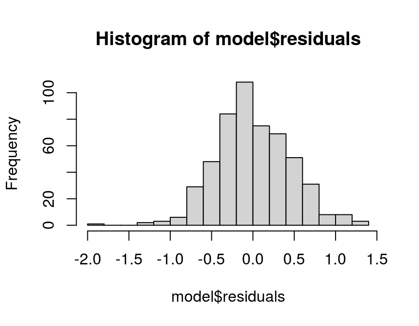

Since the shape of the histogram resembles the famous bell shape of a normal distribution, this looks pretty normal to me. However, there are more formal ways to test for normality, which are required by a more sophisticated audience than me…

• The Shapiro-Wilk test is considered to be a very reliable test for normality. It is implemented in the shapiro.test function of the stats package:

shapiro.test(model$residuals)

## 
##  Shapiro-Wilk normality test
## 
## data:  model$residuals
## W = 0.99258, p-value = 0.01031

The low p-value indicates that the null hypothesis of a normal distribution is not rejected at the 1 percent level.

• The Anderson–Darling test is also a popular normality test. It also has the advantage that it can be applied to other distributions as well. To test for normal distributions in R, the ad.test function of the nortest package can be used:

library(nortest)

ad.test(model$residuals)

## 
##  Anderson-Darling normality test
## 
## data:  model$residuals
## A = 0.86991, p-value = 0.02559

The low p-value also indicates that the null hypothesis of a normal distribution is not rejected at the 2.56 percent level.

• The Jarque-Bera test tests whether the skewness and kurtosis of a model’s residuals match the expected values for normal distribution. In R the function jarque.bera.test of the tseries packages and the function jarque.test in the moments package are, among others, implementations of this test:

library(tseries)

jarque.bera.test(model$residuals)

## 
##  Jarque Bera Test
## 
## data:  model$residuals
## X-squared = 7.1519, df = 2, p-value = 0.02799

Again, the low p-value of the Jarque-Bera test indicates that the skewness and kurtosis of the test are not significantly different from their expected values for normal distribution. Thus, the distribution of the model residuals seems statistically not different from a normal distribution.

Antidotes

In order to deal with non-normality in the errors, you could consider the following options:

• Use the log of the dependent variable for you regression.
• For time series data use the first difference of the dependent variable, because you might have a stationarity issue.
• Use a different estimator. For example, if your dependet varible can only have positive values, you might be better off with a generalised linear model, which assumes Gamma-distributed errors. Or for count data you might want to use a Poisson estimator etc.

Tests

• Eyeball test: One way to check for heteroskedasticity is to look at a plot, where the absolute values of the residuals - or the squared residuals - are plotted against the regressors of the model. If the size of the absolute (or squared) errors appears to vary with the size of a regressor, this migth indicate heteroskedasticity.

# Create plot input
hetsk_data <- cbind(abs(model$residuals), model$model[, -1])

# Scatterplot matrix
plot(hetsk_data)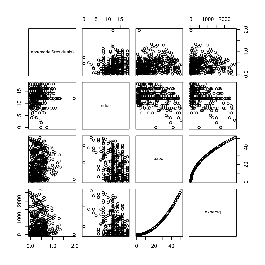

By looking at the first row of the above scatter plot we might notice that the absolute errors seem to be larger for higher values of educ and lower for higher values of expersq. This might warrant to test this more formally.

• The Breusch-Pagan test is implemented in the function pbtest both of the AER and lmtest package and tests whether the variance of a model’s residuals dependents on the values of the regressors.

library(AER)

bptest(model)

## 
##  studentized Breusch-Pagan test
## 
## data:  model
## BP = 19.84, df = 3, p-value = 0.0001832

• The White test regresses the squared residuals from the original regression model onto a set of regressors that contain the original regressors along with their squares and cross-products. Since it builds on the Breusch-Pagan test, the bptest can be used to perform the White test by adding the dependend variables and its squared values to the estimation formula:

bptest(model, ~ lwage + I(lwage^2), data = wage1)

## 
##  studentized Breusch-Pagan test
## 
## data:  model
## BP = 319.9, df = 2, p-value < 2.2e-16

• The Goldfeld-Quandt test basically devides the sample into two groups with low and high values of an explanatory variable and compares the variances of two submodels. If the variances differ, this indicates heteroskedasticity. It is implemented in the function gqtest of the lmtest package:

library(lmtest)

gqtest(model)

## 
##  Goldfeld-Quandt test
## 
## data:  model
## GQ = 0.74514, df1 = 259, df2 = 259, p-value = 0.9909
## alternative hypothesis: variance increases from segment 1 to 2

Note that this test has a series of drawbacks, which is why it is not used very often. The Breusch-Pagan and White test are used much more frequently.

Antidotes

• If the basic structure of heteroskedasticity is unknown - as is usually the case - use heteroskedasticity robust standard errors.
• If the researcher feels that the structure of heteroskedasticity can be estimated, use the feasible GLS estimator

Hausman test

A popular method to test for correlation between explanatory variables and the error term is the Hausman test. It basically tests whether the results of the IV estimator are significantly different from the OLS estimator. To illustrate this, let’s use the wage2 dataset from the wooldridge package and, again, estimate a basic Mincer earnings function as described above. However, this time we add IQ as a measure of ability. But since it is assumed that the measure is correlated with the error term, we use an additional measure of ability, KWW, as an instrument for IQ.

library(dplyr)
library(wooldridge)
data("wage2")

# Add squared experience "expersq"
wage2 <- wage2 %>%
  mutate(expersq = exper^2)

# IV estimator
iv_model <- ivreg(lwage ~ educ + exper + expersq + IQ | KWW + educ + exper + expersq,
                  data = wage2)

The summary function of the ivreg object, performs the Hausman test automatically. We only have to add the argument diagnostics = TRUE.

summary(iv_model, diagnostics = TRUE)

## 
## Call:
## ivreg(formula = lwage ~ educ + exper + expersq + IQ | KWW + educ + 
##     exper + expersq, data = wage2)
## 
## Residuals:
##       Min        1Q    Median        3Q       Max 
## -2.097500 -0.256972  0.005075  0.274838  1.284012 
## 
## Coefficients:
##              Estimate Std. Error t value Pr(>|t|)    
## (Intercept) 4.5137035  0.2437555  18.517  < 2e-16 ***
## educ        0.0096496  0.0155761   0.620    0.536    
## exper       0.0144617  0.0145717   0.992    0.321    
## expersq     0.0001935  0.0006100   0.317    0.751    
## IQ          0.0191398  0.0038791   4.934 9.54e-07 ***
## 
## Diagnostic tests:
##                  df1 df2 statistic  p-value    
## Weak instruments   1 930     77.13  < 2e-16 ***
## Wu-Hausman         1 929     15.63 8.26e-05 ***
## Sargan             0  NA        NA       NA    
## ---
## Signif. codes:  0 '***' 0.001 '**' 0.01 '*' 0.05 '.' 0.1 ' ' 1
## 
## Residual standard error: 0.4231 on 930 degrees of freedom
## Multiple R-Squared: -0.004854,   Adjusted R-squared: -0.009176 
## Wald test: 36.38 on 4 and 930 DF,  p-value: < 2.2e-16

The (Wu-)Hausman test statistic has a very low p-value and, hence, the test rejects the null of no correcation between IQ and the error term in this example.

Sargan test

The Sargan test checks whether an instrument is correlated with the errors, which should not be the case for good instruments. In the example above, the test statistic of the Sargan test is NA. This is to be expected, because we use one instrument for one endogenous regressor and the mathematical properties of the test require us to have at least one instrument more than endogenous regressor. So, if we use more instruments than endogenous regressors, the system would be identified and we would be able to obtain a test statistic. A low statistic (with rather high p-value) would indicate that the instrument is uncorrelated with the error term.

To be continued… (January 2020)