An Introduction to Ordinary Least Squares (OLS) in R

The method of least squares

To understand the basic idea of the method of least squares, imagine you were an astronomer at the beginning of the 19th century, who faced the challenge of combining a series of observations, which were made with imperfect instruments and at different points in time.¹ One day you draw a scatter plot, which looks similar to the following:

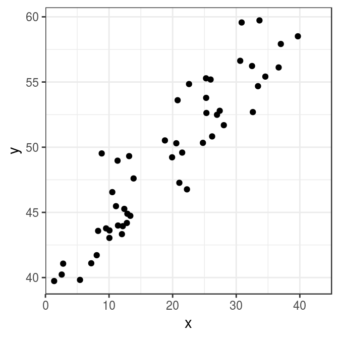
As you look at the plot, you notice a clear pattern in the data: The higher the value of variable \(x\), the higher the value of variable \(y\). But the points do not lie on a single line, although we would expect that behaviour from an astronomical law of nature, because such a law should be invariant to any unrelated factors such as when, where, or how we look at it. But since we made our observations under imperfect conditions, measurement errors prevent the points from lying on the expected straight line. Instead, they seem to be scatterd around an imaginary straight line, which goes from the bottom-left to the top-right of the plot.

From an astronomical perspective, our main interest in the graph is the slope of that imaginary line, because it describes the strength of the relationship between the variables. If the slope is steep \(y\) will change considerably after a change in \(x\). If the slope is rather flat, \(y\) will change only moderately. Under perfect conditions with no measurement errors we could just connect the points in the graph and directly measure the slope of the resulting line. But since there are errors in the data, this approach is not feasible.

This is where the method of least squares comes in. Basically, this method is nothing else than a mathematical tool, which helps in finding the imaginary line through the point cloud. You could think of it as trying out all possible ways to draw a line through the scatter plot until you have found the line, which describes the data in the best way. But what does best mean in this context? You would need some kind of normative criterium to describe which line fits the data better than another.

A quite intuitive approach to this problem would be to search for the line, which minimises the measurement errors in our data. So, we could draw a random line through the point cloud and calculate the sum of squared errors for it – i.e. the sum over the squared differences between the points and the line. After we have done this for all possible choices, we would choose the line that produces the least amount of squared errors. This is also what gives the method its name, least squares.

The only problem with this approach is that there are infinitely many ways to draw a line through the plot. So, in practice, we would not be able to find the best line just by trial and error. Luckily, there is an elegant mathematical way to do it, which Legendre and Gauss proposed independently of each other at the beginning of the 19th century. They reduced the challenge of drawing infinitely many lines and calculating their errors to a relatively simple mathematical problem² that can be solved with basic algebra. Their least squares approach has become a basic tool for data analysis in different scientific disciplines. It is so common now that it is meanwhile called ordinary least squares (OLS) and should be implemented in every modern statistical software package, including R.

Creating an artificial sample

Before we apply OLS in R, we need a sample. For convenience, I use the artificial sample from above, which consists of 50 observations from the following relationship: \[y_i = 40 + 0.5 x_i + e_i,\] where \(e_i\) is normally distributed with zero mean and variance 4, i.e. \(e_i \sim N(0, 4)\), and \(x_i\) is simulated from a uniform distribution between 1 and 40, which can be written as \(x_i \sim U(1, 40)\). So, if there were no measurement errors, variable \(y\) would lie on a straight line and increase by 0.5 when \(x\) increases by 1 and take the value 40 if \(x\) was zero.

The following R code produces the sample

# Reset random number generator for reproducibility
set.seed(1234)

# Total number of observations
N <- 50

# Simulate variable x from a uniform distribution
x <- runif(N, 1, 40)

# Simulate y
y <- 40 + .5 * x + rnorm(N, 0, 2)

# Note that the 'rnorm' function requires the standard deviation instead
# of the variance of the distribution. So, we have to enter 2 in order
# to draw from a normal distribution with variance 4.

# Store data in a data frame
ols_data <- data.frame(x, y)

If you want to be sure, execute plot(ols_data) to check whether the data is really the same as above.

OLS regression in R

The standard function for regression analysis in R is lm. Its first argument is the estimation formula, which starts with the name of the dependent variable – in our case y – followed by the tilde sign ~. Every variable name, which follows the tilde, is used as an explanatory variable and has to be separated from the other predictors with a plus sign +. But since we just have one explanatory variable, we just use x after the tilde. Next, we have to specify, which data R should use. This is done by adding data = ols_data as a further argument to the function. After that, we can estimate the model, save its results in object ols, and print the results in the console.

# Estimate the model and same the results in object "ols"
ols <- lm(y ~ x, data = ols_data) 

# Print the result in the console
ols

## 
## Call:
## lm(formula = y ~ x, data = ols_data)
## 
## Coefficients:
## (Intercept)            x  
##     39.3411       0.5107

As you can see, the estimated coefficients are quite close to their true values. Also note that we did not have to specify an intercept term in the formula, which describes the expected value of \(y\) when \(x\) is zero. The inclusion of such a term is so usual that R adds it to every equation by default unless specified otherwise.

However, the output of lm might not be enough for a researcher who is interested in test statistics to decide whether to keep a variable in a model or not. In order to get further information like this, we use the summary function, which provides a series of test statistics when printed in the console:

summary(ols)

## 
## Call:
## lm(formula = y ~ x, data = ols_data)
## 
## Residuals:
##     Min      1Q  Median      3Q     Max 
## -3.9384 -1.6412 -0.4262  1.4503  5.6626 
## 
## Coefficients:
##             Estimate Std. Error t value Pr(>|t|)    
## (Intercept) 39.34110    0.66670   59.01   <2e-16 ***
## x            0.51066    0.03054   16.72   <2e-16 ***
## ---
## Signif. codes:  0 '***' 0.001 '**' 0.01 '*' 0.05 '.' 0.1 ' ' 1
## 
## Residual standard error: 2.2 on 48 degrees of freedom
## Multiple R-squared:  0.8535, Adjusted R-squared:  0.8504 
## F-statistic: 279.6 on 1 and 48 DF,  p-value: < 2.2e-16

Please, refer to an econometrics textbook for a precise explanation of the information shown by the summary function for the output of lm. A more in-depth treatment of it would be beyond the scope of this introduction.

Finally, we can also draw the line, which results from the estimation of our model, into the graph from above. Given the method of least squares, which we used to calculate the slope and position of the line, this is our best estimate of the relation between \(y\) and \(x\). Neat, isn’t it?

library(ggplot2)

ggplot(data, aes(x = x, y = y)) +
  geom_point() +
  geom_smooth(method = "lm", se = FALSE) +
  scale_x_continuous(limits = c(0, 45), expand = c(0, 0)) +
  theme_bw()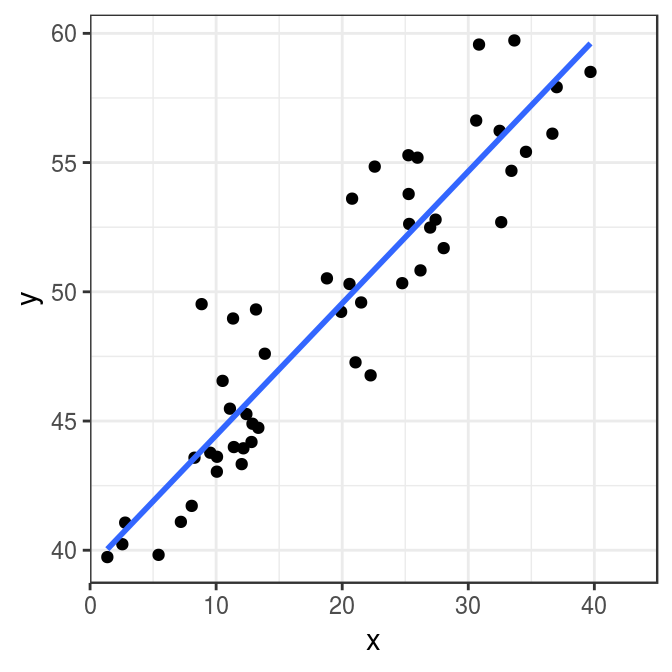

Congratulations! You just estimated a regression model. Now I would highly recommend to TEST IT.

Annex: Excluding the intercept term

If you wanted to estimate the above model without an intercept term, you have to add the term -1 or 0 to the formula:

# Estimate the model
ols_no_intercept <- lm(y ~ -1 + x, data = ols_data)

# Look at the summary results
summary(ols_no_intercept)

## 
## Call:
## lm(formula = y ~ -1 + x, data = ols_data)
## 
## Residuals:
##     Min      1Q  Median      3Q     Max 
## -25.025  -4.318   8.595  22.068  36.850 
## 
## Coefficients:
##   Estimate Std. Error t value Pr(>|t|)    
## x   2.1044     0.1209    17.4   <2e-16 ***
## ---
## Signif. codes:  0 '***' 0.001 '**' 0.01 '*' 0.05 '.' 0.1 ' ' 1
## 
## Residual standard error: 18.67 on 49 degrees of freedom
## Multiple R-squared:  0.8607, Adjusted R-squared:  0.8579 
## F-statistic: 302.7 on 1 and 49 DF,  p-value: < 2.2e-16

As you can see, the estimated coefficient value for \(x\) differs significantly from its true values. Hence, it is important to be careful with restricting the intercept term, unless there is a good reason to assume that it has to be zero.