Network Summary Statistics
with tags igraph networks network-analysis -If a network is small, it can be easily summarised by its graph or a figure. But once a network reaches a certain size, it becomes more meaningful to use more formal summary statistics in order to describe its features. This post covers some basic network summary statistics as presented in Jackson (2008). The metrics are based on the concept of centrality, which describes the importance of a node in a given network of nodes.
For this illustration I use the artificial data set generated in my post on network analysis.
Degree
The degree of a node is the number of its connections. The degree function calculates this number for each node of a graph. The node with the highest number is the node with the highest number of connections.
# Load package
library(igraph)

# Obtain degrees
g_degree <- degree(graph_df)

g_degree
## a b c d e f g h i j k l m n o p q r s t u v w x y z
## 12 20 18 11 19 16 16 16 13 14 16 10 17 15 17 12 16 18 13 13 15 15 14 19 15 20The degree is of a node is an insteresting metric to identify the most connected nodes of a network. However, if the structure of a network is of interest, the degree distribution can be an informative metric. It describes the relative frequencey of nodes that have different degrees. In that way it is a histogram of degrees.
hist(g_degree)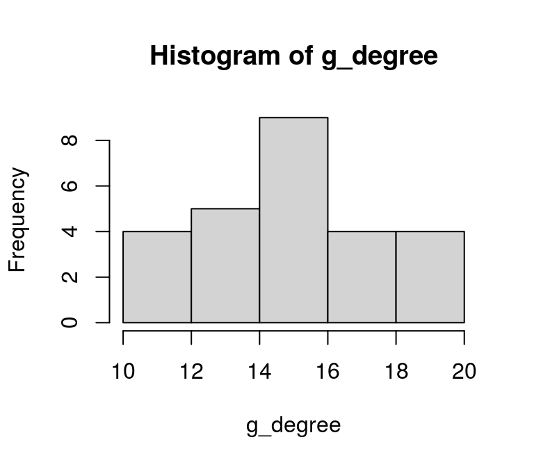
This histogram might not look very informative, which is partly due to the way the artificial network was constructed. However, as the number of nodes of a real life network increases, this distribution can become very imformative. Note that in many cases it is beneficial to obtain the distribution of the log-degree.
Let’s explore this by looking at a larger network, that can be generated with the igraph package. More precisely, we create a scale-free:
# From the example of sample_degseq

# Pre-specify the degrees of the nodes according to the
# power law
degs <- sample(1:100, 1000, replace=TRUE, prob = (1:100)^-2)

# Check if degrees sum up to an even number
# if not, add 1 to the first node to make the sum even
if (sum(degs) %% 2 != 0) {
  degs[1] <- degs[1] + 1
}

# Create random graph
g_large <- sample_degseq(degs, method = "vl")

# Calculate degree
deg_large <- degree(g_large)

# Histogram of the degree
hist(deg_large)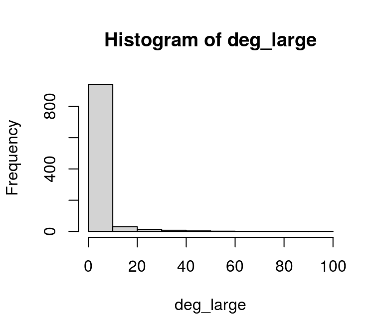
The degree distribution showes that most nodes have less than 10 connections and there are a few with more than 80. If we did not already know that the degree distribution follows a power-law, this might be a sign that we are dealing with such a network. A look at the log-degree distribution might support this suspition as well:
hist(log(deg_large))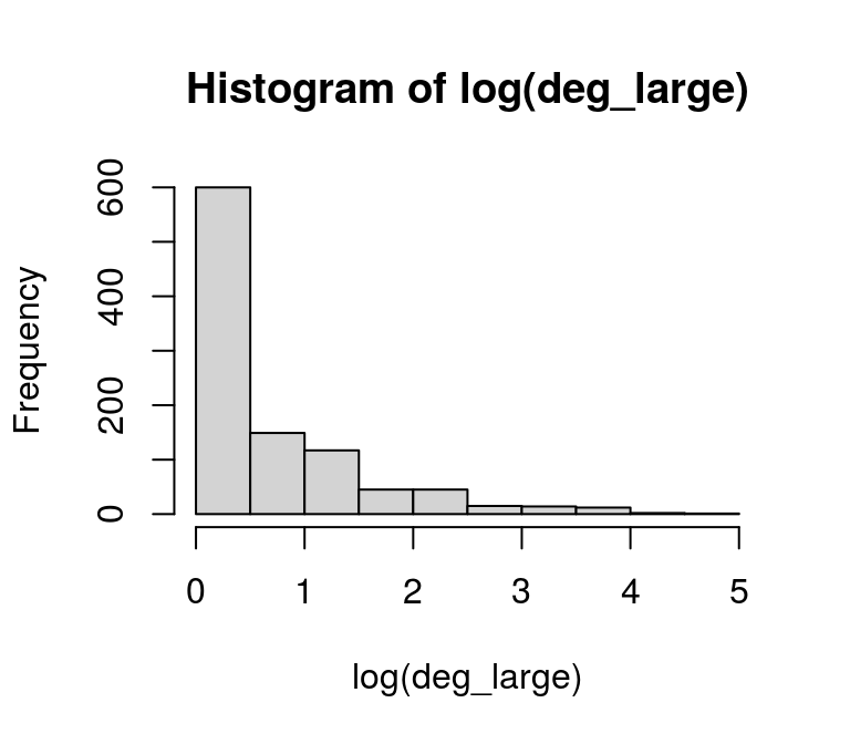
Closeness
Closeness centrality describes how close a given node is to any other node. It is usually defined as the inverse of the average of the shortest path between a node and all other nodes. Therefore, shorter paths between a node and any other node in the graph imply a higher value of the ratio.
g_close <- closeness(graph_df)

round(g_close, 2)
## a b c d e f g h i j k l m n o p
## 0.02 0.03 0.03 0.02 0.03 0.03 0.03 0.03 0.03 0.03 0.03 0.03 0.03 0.03 0.03 0.03
## q r s t u v w x y z
## 0.03 0.03 0.03 0.03 0.03 0.03 0.03 0.03 0.03 0.03In constrast to the degree of a node, which describes the number of its direct connections, its closeness provides an idea of how well a node is indirectly connected via other nodes.
Betweenness
Freeman (1977) proposes betweenness centrality as the number of shortest paths passing through a node. A higher value of a node impilies that other nodes are well connected through it.
g_betw <- betweenness(graph_df)

round(g_betw, 2)
## a b c d e f g h i j k l m
## 3.22 9.75 8.33 1.48 9.76 7.67 6.86 4.60 2.57 4.16 6.56 1.61 5.38
## n o p q r s t u v w x y z
## 4.93 6.95 3.85 6.83 8.05 3.81 3.53 5.05 5.72 3.13 11.09 6.21 10.90Eigenvector centrality
Eigenvector centrality (Bonabeau, 1972) is based on the idea that the importance of a node is recusively related to the importance of the nodes pointing to it. For example, your popularity depends on the popularity of your friends, whose popularity depends on their friends etc. Therefore, this measure is also self-referential in the sense that a node’s centrality depends on the centrality of another node, whose centrality depends the first node. A higher value of eigenvector centrality implies that a node’s neighbours are more prestigious than the neighbours of other nodes.
g_eigen <- eigen_centrality(graph_df)

round(g_eigen$vector, 2)
## a b c d e f g h i j k l m n o p
## 0.59 1.00 0.88 0.59 0.93 0.76 0.79 0.85 0.65 0.72 0.78 0.51 0.89 0.75 0.85 0.59
## q r s t u v w x y z
## 0.79 0.89 0.65 0.66 0.76 0.76 0.72 0.91 0.72 1.00Centrality measures with decay factors
A further group of centrality measures uses decay factors to take into account that links with more distant neighbours should be less influential in the calculation of a node’s centrality. The following mesures belong to this group:
- Decay centrality is based on closeness
- Katz prestige-2 as a special case of Bonacich centrality as implemented with
power_centrality
These are useful measures as well, however, they require the researcher to specify additional variables such as the decay factor, which can have a substantial impact on the results. While one specification might lead to results that are similar to the degree distribution, since it favours the close neighbourhood of a node, another specification could givs more weight to longer paths.
Relationships between the measures
To conclude this post, let’s look at the relationships between the different network measures. For this we can use scatterplot matrices.
Small network
# Collect the different centrality measures in a data frame
centr_small <- data.frame(degree = g_degree,
                          closeness = g_close,
                          betweenness = g_betw,
                          eigenvalue = g_eigen$vector)

# Scatterplot matrix
pairs(centr_small)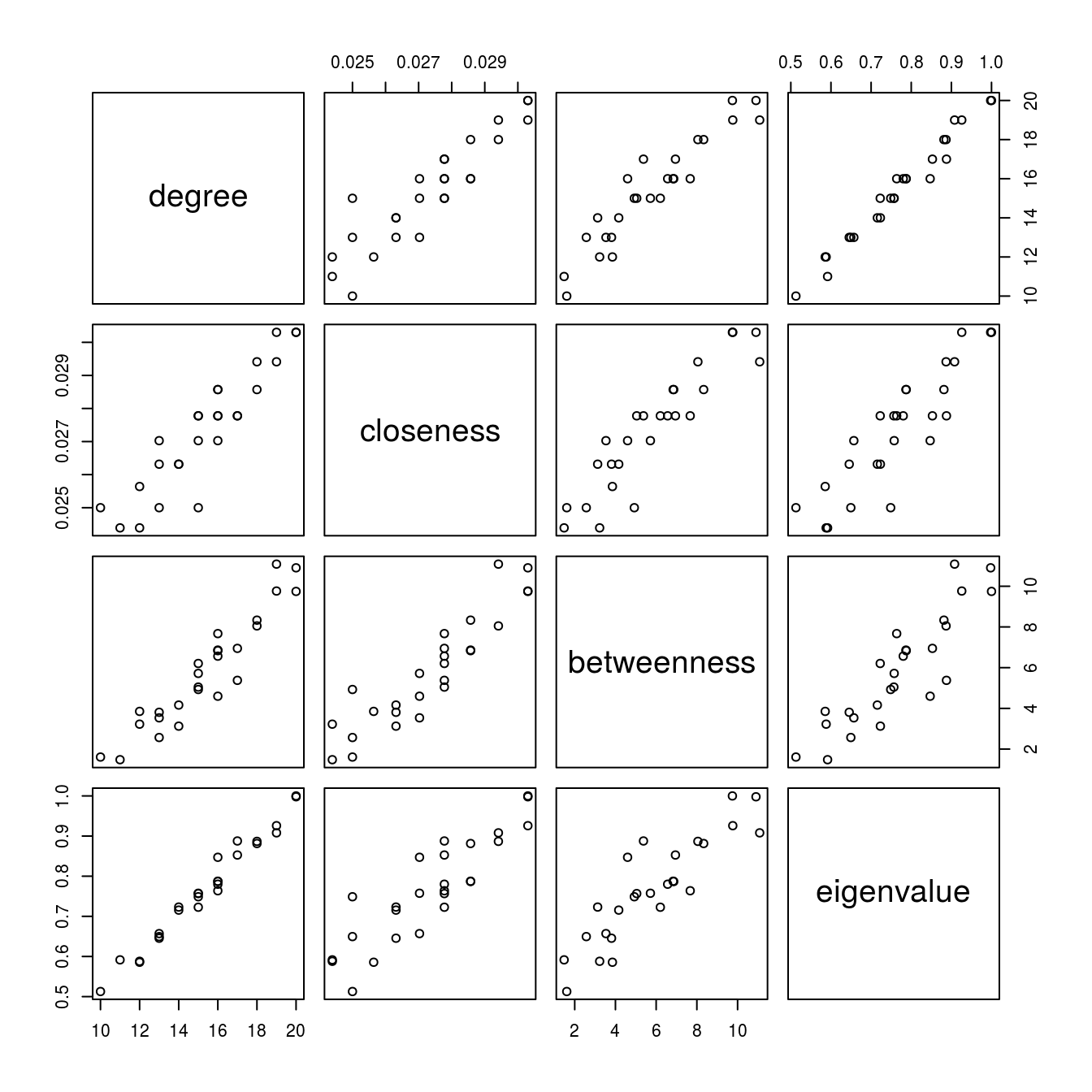
For the small graph the scatterplot matrix of the different centrality measures suggest that they have a linear relationship and, hence, each measure provides more or less the same information. However, this is probably the result of the way the small network was generated in the first place.
Large network
Looking at the scatterplot matrix of the centrality measures of the larger network provides a different picture:
# Collect the different centrality measures in a data frame
centr_large <- data.frame(degree = degree(g_large),
                          closeness = closeness(g_large),
                          betweenness = betweenness(g_large),
                          eigenvalue = eigen_centrality(g_large)$vector)

# Scatterplot matrix
pairs(centr_large)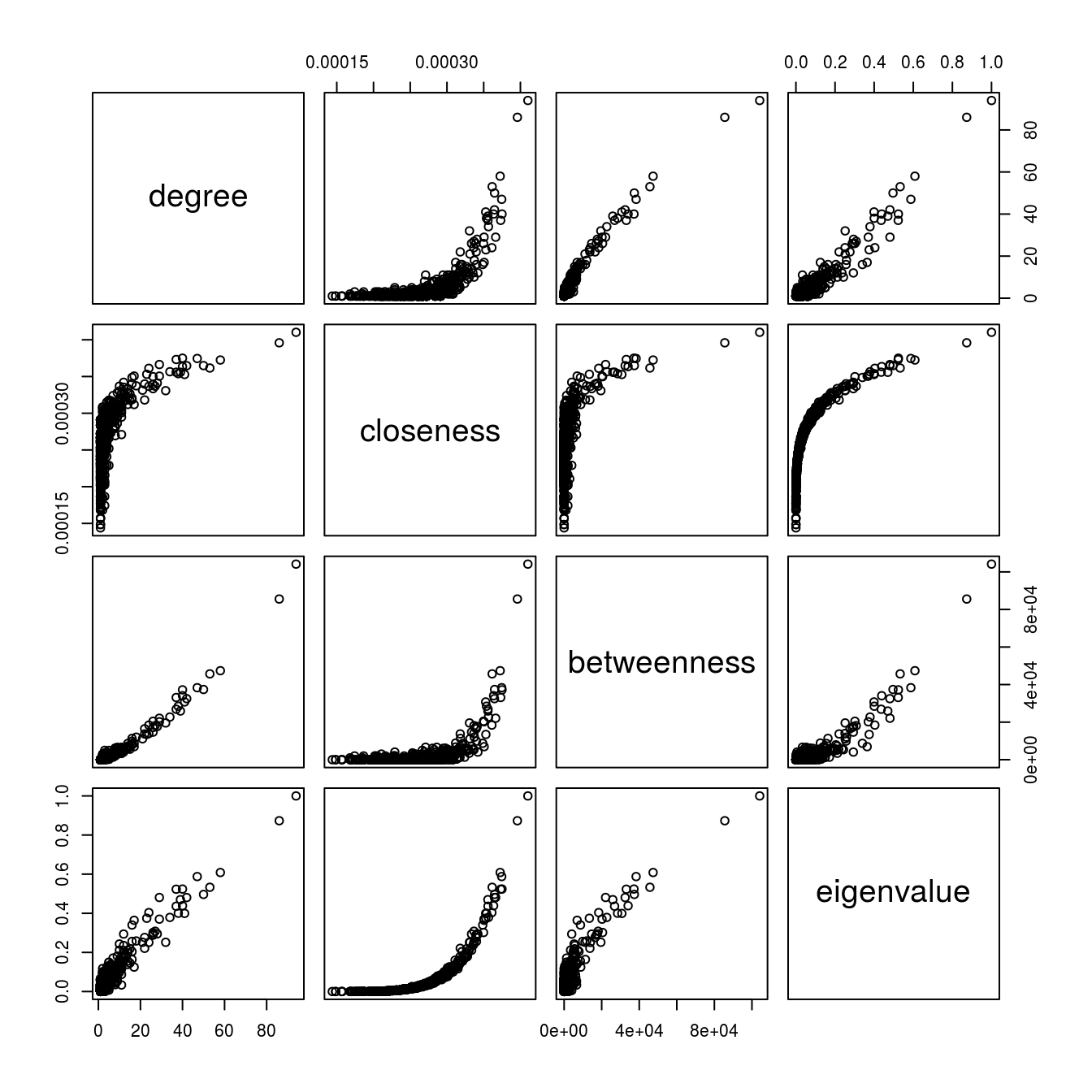
For example, although the degree and eigenvalue centrlity exhibit a quite linear relationship, the relationship between degree centrality and closeness seems to be non-linear.
References
Bonabeau, E. (1972). Factoring and weighting approaches to status scores and clique identification. Journal of Mathematical Sociology 2, 113-120.
Csardi G., & Nepusz, T. (2006). The igraph software package for complex network research, InterJournal Complex Systems, 1695.
Freeman, L. C. (1977). A set of measures of centrality based on betweenness. Sociometry 40, 35-41.
Jackson, M. O. (2008). Social and economic networks. Princeton: University Press.