Reproduction: Hochmuth, P., & Petz, N. (2026). On the persistence of services inflation and the price of services relative to goods.
with tags r bvartools vecm error-correction inflation relative-prices hicpThis post reproduces results from Hochmuth and Petz (2026) with bvartools, including the brief’s three descriptive charts: the composition of euro area inflation, and the relative price of services in the euro area and the United States.
The model
Let \(s_t = 100 \ln P^s_t\) and \(n_t = 100 \ln P^n_t\) be the log price indices of services and NEIG. The paper fixes the cointegrating vector at \(\beta = (1, -1)'\), so that \(\beta' y_t = s_t - n_t\) is the log relative price of services, and assumes that it follows a linear trend:
\[s_t - n_t = \mu + \delta t + z_t,\]
where \(z_t\) is stationary. The trend allows the two price indices to grow at different rates in the long run, and \(z_t\) is the deviation from it, the relative-price gap.
The model is estimated in two stages. The first is an OLS regression of the relative price on a constant and a trend, whose residual \(\hat{z}_t\) is the estimated gap. The second is a VECM that uses \(\hat{z}_{t-1}\) as its error correction term,
\[\Delta y_t = \kappa + \alpha \hat{z}_{t-1} + \Gamma \Delta y_{t-1} + \varepsilon_t, \quad \varepsilon_t \sim N(0, \Sigma),\]
with \(\Delta y_t = (\Delta s_t, \Delta n_t)'\). The loadings \(\alpha = (\alpha_s, \alpha_n)'\) say how services and NEIG inflation respond to a gap. The paper puts independent standard normal priors on \(\kappa\), \(\alpha\) and \(\Gamma\), and an inverse Wishart prior on \(\Sigma \sim IW(4, 0.01 I)\).
Since \(\hat{z}_{t-1}\) is data once the first stage is done, the second stage is a VAR(1) in \(\Delta y_t\) with one exogenous regressor, which is how it is estimated below.
The data
The paper uses monthly harmonised indices of consumer prices (HICP) for the euro area (changing composition) from Eurostat data set prc_hicp_minr, from January 1996 to June 2026, which the eurostat package downloads. They are seasonally adjusted with X-13ARIMA-SEATS from the seasonal package and averaged to quarters. The code uses the following packages:
library("bvartools")
library("dplyr")
library("knitr")
library("magrittr")
library("seasonal")
library("tibble")
library("tidyr")
The data set is the first that Eurostat publishes under the new ECOICOP version 2, and the vintage of October 2026 has no euro area index before December 1999, although the paper says it started in January 1996 when it was downloaded in August. The ECB Data Portal still has the old ECOICOP version 1 indices, which start in 1996 and which the ecb package downloads, so the missing months are filled in with their month-on-month growth rates. The ECB’s NEIG index itself has a hole from January 1997 to November 2000, which its published annual rates of change fill: \(P_t = P_{t-12} (1 + \pi^{yoy}_t / 100)\). Since those rates have only one decimal, each year rebuilt that way is off by at most 0.05%.
library("ecb")
library("eurostat")

# Eurostat, ECOICOP ver. 2: services, NEIG and goods, 2025 = 100
hicp_filters <- list(geo = "EA",
                     unit = "I25",
                     coicop18 = c("SERV", "IGD_NNRG", "GD"))

hicp_new <- get_eurostat("prc_hicp_minr",
                         time_format = "raw",
                         cache = FALSE,
                         filters = hicp_filters) %>%
  transmute(month = as.character(time),
            series = coicop18,
            index = values) %>%
  filter(month <= "2026-06")

# ECB, ECOICOP ver. 1: index levels (INX) and annual rates (ANR), 1996-2001
hicp_old <- get_data("ICP.M.U2.N.SERV00+IGXE00+GOODS0.4.INX+ANR",
                     filter = list(startPeriod = "1996-01",
                                   endPeriod = "2001-12")) %>%
  transmute(month = obstime,
            series = recode_values(icp_item,
                                   "SERV00" ~ "SERV",
                                   "IGXE00" ~ "IGD_NNRG",
                                   "GOODS0" ~ "GD"),
            suffix = icp_suffix,
            value = obsvalue) %>%
  pivot_wider(names_from = suffix, values_from = value)

# Fill a missing index level from the same month a year earlier and the
# annual rate: chained from 1996, I_t = I_{t-12} (1 + ANR_t / 100)
hicp_old <- hicp_old %>%
  mutate(calendar_month = substr(month, 6, 7)) %>%
  arrange(series, calendar_month, month) %>%
  group_by(series, calendar_month) %>%
  mutate(chained = cumprod(if_else(row_number() == 1, INX, 1 + ANR / 100)),
         INX = coalesce(INX, chained)) %>%
  ungroup()

# Back-cast each Eurostat series with the growth of its ECB counterpart
hicp_old_index <- hicp_old %>%
  select(month, series, old = INX)

hicp <- hicp_new %>%
  full_join(hicp_old_index, by = c("month", "series")) %>%
  arrange(series, month) %>%
  group_by(series) %>%
  mutate(first_month = min(month[!is.na(index)]),
         first_index = index[month == first_month],
         first_old = old[month == first_month],
         index = coalesce(index, first_index * old / first_old)) %>%
  ungroup()

hicp %>%
  pivot_wider(id_cols = month,
              names_from = series,
              values_from = index) %>%
  select(month, GD, IGD_NNRG, SERV) %>%
  write.csv("_2026_hochmuth_petz_hicp.csv", row.names = FALSE)
The result is in a small file next to this page, so that the post does not change with the next vintage:
hicp <- read.csv("_2026_hochmuth_petz_hicp.csv") %>%
  pivot_longer(-month, names_to = "series", values_to = "index") %>%
  arrange(series, month)

# X-13ARIMA-SEATS with the defaults of seasonal, series by series
hicp <- hicp %>%
  group_by(series) %>%
  mutate(index_sa = ts(index, start = c(1996, 1), frequency = 12) %>%
           seas() %>%
           final() %>%
           as.numeric()) %>%
  ungroup()

# Quarterly averages, dated by the start of the quarter: 1996.25 is 1996 Q2
prices <- hicp %>%
  mutate(year = as.integer(substr(month, 1, 4)),
         month_of_year = as.integer(substr(month, 6, 7)),
         quarter = year + (month_of_year - 1) %/% 3 / 4) %>%
  group_by(series, quarter) %>%
  summarise(index = mean(index),
            index_sa = mean(index_sa),
            .groups = "drop")
The composition of euro area inflation
Chart 1 of the brief splits euro area HICP inflation since 2018 into the contributions of energy, food including alcohol and tobacco, NEIG and services. Eurostat publishes these contributions in percentage points as data set prc_hicp_ctr, and the annual rates of headline and core inflation – the overall index excluding energy, food, alcohol and tobacco – are in prc_hicp_minr:
contribution_filters <- list(geo = "EA",
                             coicop18 = c("NRG", "FOOD", "IGD_NNRG", "SERV"))

contributions <- get_eurostat("prc_hicp_ctr",
                              time_format = "raw",
                              cache = FALSE,
                              filters = contribution_filters)

inflation_filters <- list(geo = "EA",
                          unit = "RCH_A",
                          coicop18 = c("TOTAL", "TOT_X_NRG_FOOD"))

inflation <- get_eurostat("prc_hicp_minr",
                          time_format = "raw",
                          cache = FALSE,
                          filters = inflation_filters)

# From 2018 to the brief's last observation
bind_rows(contributions, inflation) %>%
  transmute(month = as.character(time),
            series = coicop18,
            value = values) %>%
  filter(month >= "2018-01", month <= "2026-07") %>%
  pivot_wider(names_from = series, values_from = value) %>%
  select(month, FOOD, IGD_NNRG, NRG, SERV, TOTAL, TOT_X_NRG_FOOD) %>%
  arrange(month) %>%
  write.csv("_2026_hochmuth_petz_contributions.csv", row.names = FALSE)
The contributions add up to headline inflation up to rounding. The bars of a month are stacked upwards from zero where they are positive and downwards where they are negative. All charts on this page share one set of colours, with services always in blue:
colours <- c(red = "#C10016",
             blue = "#0F4C81",
             amber = "#E8A33D",
             teal = "#17807A",
             ink = "#22282E",
             grid = "#DCE1E5")

component_colours <- c(SERV = colours[["blue"]],
                       IGD_NNRG = colours[["teal"]],
                       FOOD = colours[["amber"]],
                       NRG = colours[["red"]])
contributions <- read.csv("_2026_hochmuth_petz_contributions.csv") %>%
mutate(year = as.integer(substr(month, 1, 4)),
month_of_year = as.integer(substr(month, 6, 7)),
period = year + (month_of_year - 1) / 12)
# Stack the positive contributions of a month upwards from zero, the negative
# ones downwards, services first
bars <- contributions %>%
pivot_longer(c(SERV, IGD_NNRG, FOOD, NRG),
names_to = "component",
values_to = "value") %>%
mutate(component = factor(component, levels = names(component_colours))) %>%
arrange(month, component) %>%
group_by(month, positive = value >= 0) %>%
mutate(top = cumsum(value),
bottom = top - value) %>%
ungroup()
plot(NA,
xlim = range(contributions[["period"]]),
ylim = c(-4, 12),
xlab = "",
ylab = "Contribution to HICP inflation in %",
main = "HICP components")
grid(col = colours[["grid"]], lty = 1)
rect(bars[["period"]] - 0.035,
bars[["bottom"]],
bars[["period"]] + 0.035,
bars[["top"]],
col = component_colours[as.character(bars[["component"]])],
border = NA)
lines(contributions[["period"]],
contributions[["TOTAL"]],
lwd = 1.5,
col = colours[["ink"]])
lines(contributions[["period"]],
contributions[["TOT_X_NRG_FOOD"]],
lwd = 1.5,
lty = 2,
col = colours[["ink"]])
abline(h = 0, col = colours[["ink"]])
legend("topleft",
legend = c("Energy",
"Food including alcohol and tobacco",
"Non-energy industrial goods",
"Services",
"HICP inflation in %",
"Core inflation in %"),
fill = c(rev(component_colours), NA, NA),
border = NA,
lty = c(NA, NA, NA, NA, 1, 2),
col = colours[["ink"]],
bty = "n",
cex = 0.8)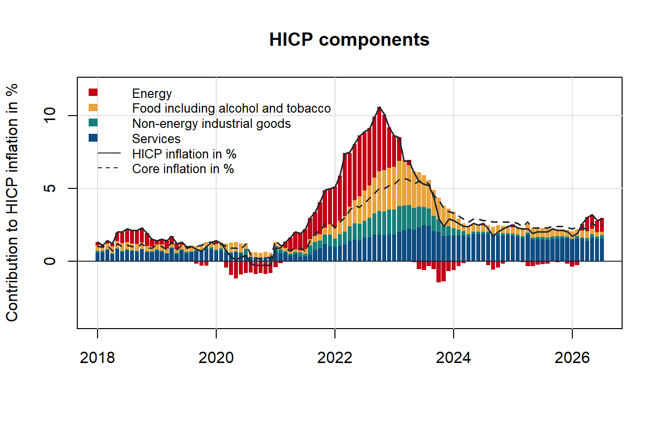
The chart matches the published one. Headline inflation peaked at 10.6% in October 2022, when energy alone contributed 4.44 percentage points. The contribution of services rose more slowly and peaked later, at 2.47 points in July 2023, and has receded more slowly than the others: in July 2026 it still accounted for 1.55 of 2.9 points, more than half of headline inflation, while energy, which had subtracted from inflation for most of 2023 to 2025, was adding 0.94 points again.
The price of services relative to goods
Chart 2 of the brief shows the price of services relative to NEIG and to overall goods as a four-quarter moving average, indexed to 100 in the first quarter of 2000, together with a log-linear trend fitted over 1996 to 2019 and extrapolated from there. The moving average removes the seasonal pattern, so the chart works with quarterly averages of the unadjusted indices:
relative_prices <- prices %>%
  select(series, quarter, index) %>%
  pivot_wider(names_from = series, values_from = index) %>%
  pivot_longer(c(IGD_NNRG, GD),
               names_to = "goods",
               values_to = "goods_index") %>%
  arrange(goods, quarter) %>%
  group_by(goods) %>%

  # Four-quarter moving average, indexed to Q1 2000 = 100
  mutate(ratio = SERV / goods_index,
         price = (ratio + lag(ratio) + lag(ratio, 2) + lag(ratio, 3)) / 4,
         price = 100 * price / price[quarter == 2000]) %>%

  # Log-linear trend fitted over 1996-2019, extrapolated from there
  mutate(trend = exp(predict(lm(log(price) ~ quarter, subset = quarter < 2020),
                             newdata = data.frame(quarter = quarter))),
         growth = 100 * coef(lm(log(price) ~ quarter,
                                subset = quarter < 2020))[["quarter"]]) %>%
  ungroup()
ea_neig <- filter(relative_prices, goods == "IGD_NNRG")
ea_goods <- filter(relative_prices, goods == "GD")
price_range <- range(c(relative_prices[["price"]], relative_prices[["trend"]]),
na.rm = TRUE)
plot(ea_neig[["quarter"]],
ea_neig[["price"]],
type = "l",
lwd = 2,
col = colours[["teal"]],
ylim = price_range,
xlab = "",
ylab = "Relative price (Q1 2000 = 100)",
main = "Price of services relative to goods (euro area)")
lines(ea_neig[["quarter"]],
ea_neig[["trend"]],
lwd = 2,
lty = 2,
col = colours[["teal"]])
lines(ea_goods[["quarter"]],
ea_goods[["price"]],
lwd = 2,
col = colours[["amber"]])
lines(ea_goods[["quarter"]],
ea_goods[["trend"]],
lwd = 2,
lty = 2,
col = colours[["amber"]])
abline(h = 100, col = colours[["ink"]])
legend("topleft",
legend = c("Services relative to NEIG", "Services relative to goods"),
col = colours[c("teal", "amber")],
lwd = 2,
bty = "n")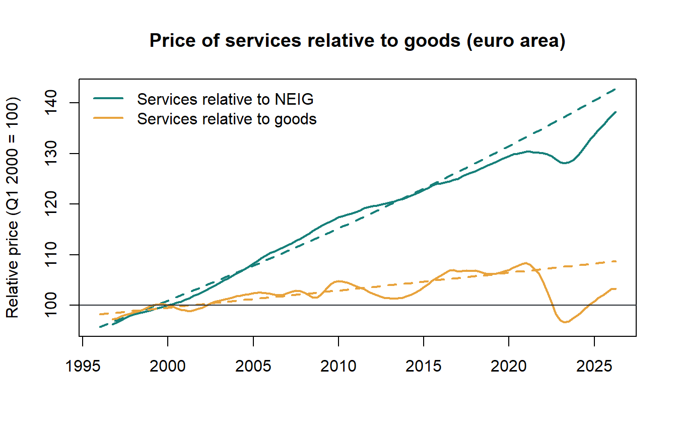
Before the pandemic services became 1.3% a year more expensive relative to NEIG, and 0.3% relative to overall goods. Both relative prices fell below their trends in 2021 and 2022. The one against overall goods fell much more, because the energy and food prices it includes rose most, and it has made up less of the loss since. In the second quarter of 2026 services relative to NEIG are 3.2% below the extrapolated trend, which the brief puts at 3.5%, and relative to overall goods 5% below it.
The euro area series is short, so the brief turns to post-war US data to ask whether such a trend survives large shocks. Chart 3 is the price of services relative to commodities in the US consumer price index for all urban consumers (CPI-U), series CUUR0000SAS and CUUR0000SAC of the Bureau of Labor Statistics. FRED, the database of the Federal Reserve Bank of St. Louis, carries both, and the alfred package downloads them:
library("alfred")

us_services <- get_fred_series("CUUR0000SAS", "CUUR0000SAS")
us_commodities <- get_fred_series("CUUR0000SAC", "CUUR0000SAC")

full_join(us_services, us_commodities, by = "date") %>%
  mutate(month = format(date, "%Y-%m")) %>%

  # FRED pads the years with quarterly observations with empty months
  filter(month >= "1947-01",
         month <= "2026-06",
         !is.na(CUUR0000SAS)) %>%
  select(month, CUUR0000SAS, CUUR0000SAC) %>%
  write.csv("_2026_hochmuth_petz_us_cpi.csv", row.names = FALSE)
Both indices are published quarterly until 1955 and monthly after that, and October 2025, when the federal government was shut down, is missing. Quarterly averages of what is there take care of both. The trend is fitted over the whole sample:
us_relative_price <- read.csv("_2026_hochmuth_petz_us_cpi.csv") %>%

  # Quarterly averages of the months observed
  mutate(year = as.integer(substr(month, 1, 4)),
         month_of_year = as.integer(substr(month, 6, 7)),
         quarter = year + (month_of_year - 1) %/% 3 / 4) %>%
  group_by(quarter) %>%
  summarise(services = mean(CUUR0000SAS),
            commodities = mean(CUUR0000SAC)) %>%

  # Four-quarter moving average, indexed to Q1 2000 = 100
  mutate(ratio = services / commodities,
         price = (ratio + lag(ratio) + lag(ratio, 2) + lag(ratio, 3)) / 4,
         price = 100 * price / price[quarter == 2000]) %>%

  # Log-linear trend over the whole sample since 1950
  filter(quarter >= 1950) %>%
  mutate(trend = exp(fitted(lm(log(price) ~ quarter))),
         growth = 100 * coef(lm(log(price) ~ quarter))[["quarter"]])

plot(us_relative_price[["quarter"]],
     us_relative_price[["price"]],
     type = "l",
     lwd = 2,
     col = colours[["blue"]],
     xlab = "",
     ylab = "Relative price (Q1 2000 = 100)",
     main = "Price of services relative to commodities (USA)")

lines(us_relative_price[["quarter"]],
      us_relative_price[["trend"]],
      lwd = 2,
      lty = 2,
      col = colours[["blue"]])

abline(h = 100, col = colours[["ink"]])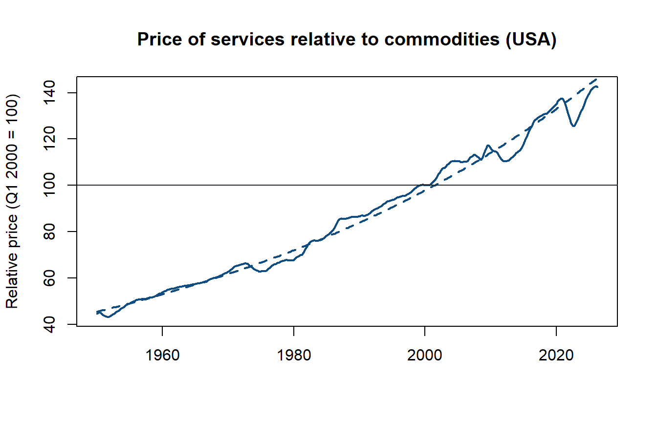
Over seventy years US services became 1.5% a year more expensive relative to commodities, and the relative price never strayed far from that trend: not in the commodity price shocks of the 1970s, not in the oil price swings of the 2000s and not in 2021 and 2022. The recent surge pushed it further below the trend than at any other time since 1950, by 9.4%, and it has since returned to within 2.7% of it, which is what the brief expects of the euro area as well. As the brief points out, the two charts are not directly comparable, since the US series compares services with commodities rather than with goods.
Estimation
A function sets up both stages for either price index, so that the benchmark and the specification with overall goods prices share the code. The first stage is lm. In the second, create_bvarmodel takes \(\hat{z}_{t-1}\) as an exogenous variable exogen with no further lags, s = 0, and add_priors sets the paper’s priors directly: a precision v_i = 1 is a standard normal prior with mean zero, and sigma = list(df = 4, scale = 0.01) is the inverse Wishart with four degrees of freedom and scale matrix \(0.01 I\). The sampler is run for 5,000 burn-in draws, and the next 20,000 are kept.
estimate_gap_model <- function(prices, other) {

  # Log prices of services (s) and of the other index (n), times 100
  y <- prices %>%
    filter(series %in% c("SERV", other)) %>%
    transmute(quarter,
              series = if_else(series == "SERV", "s", "n"),
              value = 100 * log(index_sa)) %>%
    pivot_wider(names_from = series, values_from = value) %>%
    arrange(quarter) %>%
    mutate(trend = row_number())

  # Stage 1: the relative-price gap is the residual of a linear trend
  stage_1 <- lm(s - n ~ trend, data = y)
  gap <- residuals(stage_1)

  # Stage 2: a VAR(1) in differences, with the lagged gap as exogenous
  # regressor
  dy <- ts(diff(as.matrix(y[, c("s", "n")])),
           start = y[["quarter"]][2],
           frequency = 4)

  ect <- ts(matrix(head(gap, -1), dimnames = list(NULL, "ect")),
            start = y[["quarter"]][2],
            frequency = 4)

  model <- create_bvarmodel(dy,
                            p = 1,
                            exogen = ect,
                            s = 0,
                            deterministic = "const",
                            iterations = 20000,
                            burnin = 5000)

  model <- add_priors(model,
                      coef = list(v_i = 1, v_i_det = 1),
                      sigma = list(df = 4, scale = 0.01))

  model <- add_initial_values(model, method = "ols")

  return(add_posterior_coefficients(model))
}

set.seed(20261012)

model_neig <- estimate_gap_model(prices, "IGD_NNRG")
model_goods <- estimate_gap_model(prices, "GD")summary(model_neig)##
## Bayesian VAR model with p = 1 and s = 0
##
## Endogenous variables: s, n
##
## Variable: s
##
## Mean SD Naive SD Time-series SD 2.5% 50% 97.5%
## s.l1 0.53666848 0.07921922 5.601645e-04 5.736318e-04 0.382674732 0.53679984 0.69342784 *
## n.l1 0.12547532 0.06243646 4.414924e-04 4.414924e-04 0.004790073 0.12559394 0.24943503 *
## ect.l0 -0.03260893 0.01081947 7.650522e-05 7.816906e-05 -0.053804521 -0.03253197 -0.01133798 *
## const 0.22135600 0.04045902 2.860885e-04 2.916030e-04 0.142265357 0.22148148 0.30079275 *
##
## Variable: n
##
## Mean SD Naive SD Time-series SD 2.5% 50% 97.5%
## s.l1 -0.01716661 0.10361707 7.326833e-04 7.295326e-04 -0.21867790 -0.01763009 0.18614143
## n.l1 0.71552294 0.08140224 5.756007e-04 5.756007e-04 0.55511285 0.71593500 0.87242371 *
## ect.l0 -0.01020764 0.01401152 9.907643e-05 9.907643e-05 -0.03745045 -0.01018564 0.01759145
## const 0.07280600 0.05308072 3.753374e-04 3.766556e-04 -0.03114290 0.07304980 0.17663529
##
## Variance-covariance matrix:
##
## Mean SD Naive SD Time-series SD 2.5% 50% 97.5%
## s_s 0.02752135 0.003643497 2.576342e-05 2.667543e-05 0.021308232 0.02718972 0.03559597 *
## s_n 0.01466575 0.003599254 2.545057e-05 2.627168e-05 0.008223902 0.01445134 0.02235043 *
## n_n 0.04637967 0.006205077 4.387652e-05 4.578056e-05 0.035763049 0.04578956 0.05998577 *A gap below trend, \(\hat{z}_{t-1} < 0\), raises services inflation: \(\alpha_s\) is negative and its credible interval excludes zero. The loading of NEIG inflation is negative as well, but smaller and not clearly different from zero. Since a gap closes when services inflation exceeds NEIG inflation, the NEIG response works against the adjustment.
How fast does the gap close?
To isolate the adjustment the paper simulates the model in deviations from a baseline without a gap. The intercepts and the errors then drop out, and from \(z_0 = -1\) and \(\Delta y_0 = 0\) the system evolves as
\[\Delta y_h = \alpha z_{h-1} + \Gamma \Delta y_{h-1}, \quad z_h = z_{h-1} + \Delta s_h - \Delta n_h, \quad h = 1, \ldots, H.\]
An initial gap of \(-1\) means that services are about 1% cheaper relative to NEIG than their trend implies. The cumulative contributions of services and NEIG inflation to closing it, in percent of the initial gap, are
\[C_{s,h} = 100 \sum_{j=1}^{h} \Delta s_j, \quad C_{n,h} = -100 \sum_{j=1}^{h} \Delta n_j,\]
and \(100 + 100 z_h = 100 - C_{s,h} - C_{n,h}\) is what remains of the gap after \(h\) quarters.
The draws of the coefficients are in posterior[["a"]][["coeffs"]]. Each row is one draw of \(vec(A)\), where \(A\) has one row per equation and one column per regressor, in the order summary prints them. The recursion is run for all draws at once, and the medians and the 68% credible interval are taken over the draws of each quarter:
gap_closure <- function(model, horizon = 40) {

  # Equation i's coefficient on regressor j is in column (j - 1) k + i. The
  # regressors are the lags of s and n, the error correction term and the
  # constant
  draws <- as.matrix(model[["posterior"]][["a"]][["coeffs"]])
  k <- model[["model"]][["k"]]

  gamma_ss <- draws[, 1]
  gamma_ns <- draws[, 2]
  gamma_sn <- draws[, k + 1]
  gamma_nn <- draws[, k + 2]
  alpha_s <- draws[, 2 * k + 1]
  alpha_n <- draws[, 2 * k + 2]

  # Start from z_0 = -1 and dy_0 = 0
  n_draws <- nrow(draws)
  z <- rep(-1, n_draws)
  ds <- rep(0, n_draws)
  dn <- rep(0, n_draws)
  services <- rep(0, n_draws)
  other <- rep(0, n_draws)

  paths <- vector("list", horizon)

  for (h in seq_len(horizon)) {

    ds_new <- alpha_s * z + gamma_ss * ds + gamma_sn * dn
    dn_new <- alpha_n * z + gamma_ns * ds + gamma_nn * dn

    ds <- ds_new
    dn <- dn_new
    z <- z + ds - dn

    # Cumulative contributions, in % of the initial gap
    services <- services + 100 * ds
    other <- other - 100 * dn

    paths[[h]] <- data.frame(h = h,
                             remaining = -100 * z,
                             services = services,
                             other = other)
  }

  closure <- bind_rows(paths) %>%
    group_by(h) %>%
    summarise(lower = quantile(remaining, 0.16),
              upper = quantile(remaining, 0.84),
              remaining = median(remaining),
              services = median(services),
              other = median(other))

  start <- data.frame(h = 0,
                      lower = 100,
                      upper = 100,
                      remaining = 100,
                      services = 0,
                      other = 0)

  return(bind_rows(start, closure))
}

closure_neig <- gap_closure(model_neig)
closure_goods <- gap_closure(model_goods)

closure <- bind_rows(neig = closure_neig,
                     goods = closure_goods,
                     .id = "spec")
Chart 4 of the paper shows the median of the remaining gap with its 68% credible interval, and the median contributions as bars that start at 100: the services bars point down, because higher services inflation closes the gap, and the NEIG bars point up, because higher NEIG inflation widens it. Where both contributions close the gap, as in the specification with overall goods below, the bars are stacked.
plot_closure <- function(closure, label, colour) {

  bar_colours <- adjustcolor(c(colours[["blue"]], colour), 0.45)

  plot(NA,
       xlim = range(closure[["h"]]),
       ylim = range(c(-50, 160, 100 - closure[["services"]])),
       xlab = "Quarters after the initial gap",
       ylab = "% of initial gap",
       main = "What closes the gap?")

  grid(col = colours[["grid"]], lty = 1)

  # Contributions with the same sign are stacked, opposite ones start at 100
  services_end <- 100 - closure[["services"]]
  other_start <- ifelse(sign(closure[["other"]]) == sign(closure[["services"]]),
                        services_end,
                        100)

  rect(closure[["h"]] - 0.35,
       100,
       closure[["h"]] + 0.35,
       services_end,
       col = bar_colours[1],
       border = NA)

  rect(closure[["h"]] - 0.35,
       other_start,
       closure[["h"]] + 0.35,
       other_start - closure[["other"]],
       col = bar_colours[2],
       border = NA)

  polygon(c(closure[["h"]], rev(closure[["h"]])),
          c(closure[["lower"]], rev(closure[["upper"]])),
          col = adjustcolor(colours[["ink"]], 0.2),
          border = NA)

  lines(closure[["h"]],
        closure[["remaining"]],
        col = colours[["red"]],
        lwd = 2)

  abline(h = c(0, 100), col = colours[["ink"]])

  legend("bottomleft",
         legend = c("Services", label, "Remaining gap"),
         fill = c(bar_colours, NA),
         border = NA,
         lty = c(NA, NA, 1),
         col = c(NA, NA, colours[["red"]]),
         lwd = 2,
         bty = "n")

  return(invisible(NULL))
}
plot_closure(closure_neig, label = "NEIG", colour = colours[["teal"]])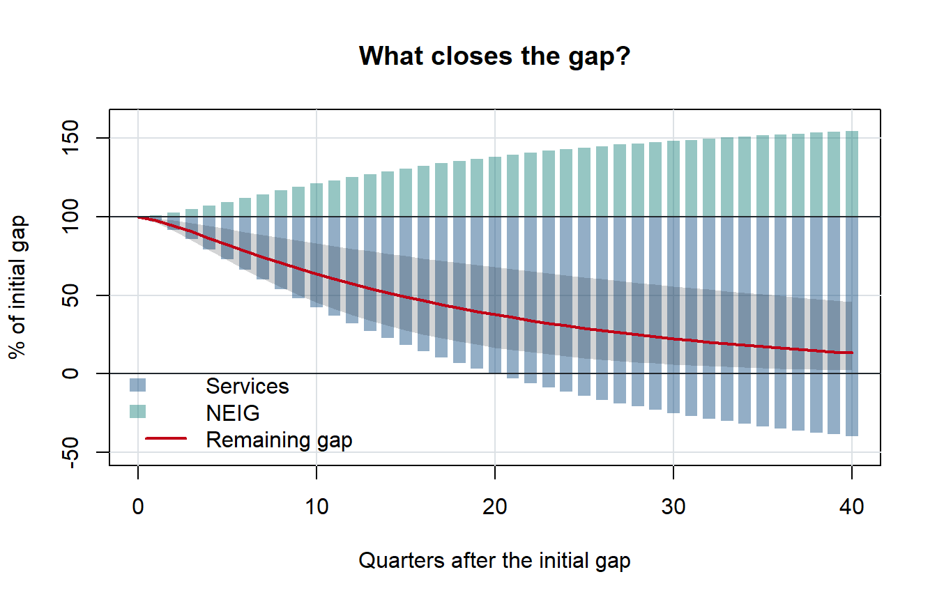
The chart is close to the published one. The remaining gap falls below 50% between quarters 14 and 15, exactly where the paper puts it, about three and a half years. At quarter 14 services inflation has closed 77 percentage points of the gap and NEIG inflation has widened it by 29, against 76 and 26 in the paper. After ten years 13% of the gap is left, as in the published chart.
closure %>%
  filter(spec == "neig", h %in% c(4, 8, 14, 15, 20, 40)) %>%
  select(h, remaining, lower, upper, services, other) %>%
  kable(digits = 1,
        row.names = FALSE,
        col.names = c("Quarter", "Remaining gap", "16%", "84%",
"Services", "NEIG"))| Quarter | Remaining gap | 16% | 84% | Services | NEIG |
|---|---|---|---|---|---|
| 4 | 86.3 | 78.6 | 94.1 | 20.7 | -7.0 |
| 8 | 70.5 | 55.1 | 86.7 | 46.2 | -16.6 |
| 14 | 51.6 | 30.7 | 76.5 | 77.4 | -29.0 |
| 15 | 49.0 | 27.7 | 75.0 | 81.7 | -30.8 |
| 20 | 37.7 | 16.7 | 67.9 | 99.9 | -38.3 |
| 40 | 13.3 | 2.1 | 45.8 | 140.0 | -54.6 |
Overall goods instead of NEIG
The same model with the overall goods index adjusts much faster:
plot_closure(closure_goods, label = "Goods", colour = colours[["amber"]])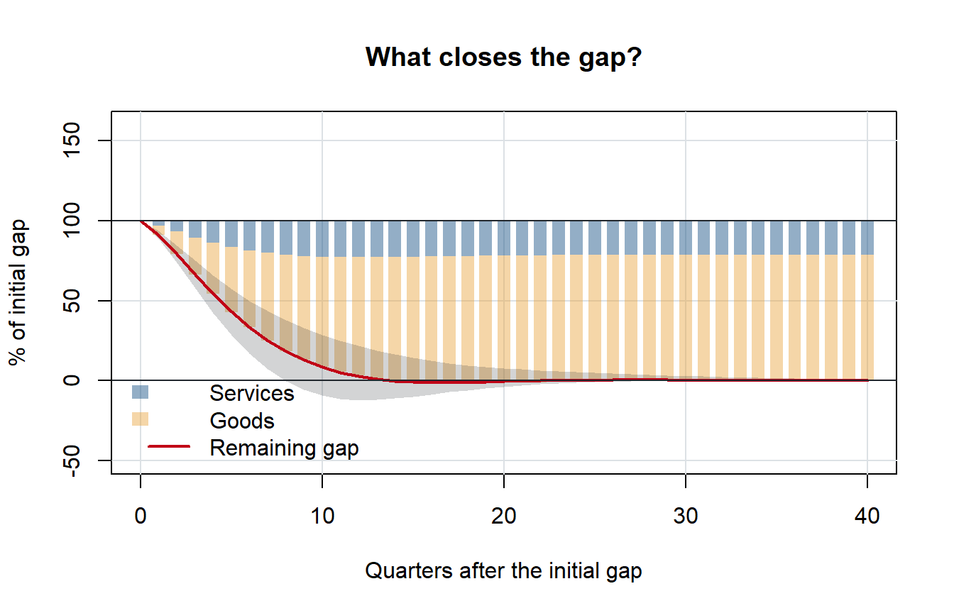
Half of the gap is closed between quarters 4 and 5, which the paper reports as about five quarters. Here, unlike in the benchmark, both components close the gap, and goods inflation does more of it: at quarter 5 services contribute 17 and goods 41 percentage points, against roughly 15 and 38 in the paper. The goods loading is positive, and its 95% credible interval excludes zero: when services are cheap relative to goods, goods inflation falls. The faster adjustment reflects the energy and food prices in the goods index, which move much more than NEIG prices and return quickly after a shock.
The post How Long Will Services Inflation in Austria Stay High? applies the same model to Austria.
Deviations from the paper
- Data before 2000. The current vintage of
prc_hicp_minrstarts in December 1999 for the euro area, so the first four years are back-cast from the ECB’s ECOICOP version 1 indices, and the NEIG index for 1997 to 2000 from its annual rates. - Data vintage. The data were downloaded on 12 October 2026 rather than 10 August, so the most recent quarters may include revisions.
- Trend sample. The paper does not say over which sample the trend of the first stage is estimated. The whole sample, 1996 Q1 to 2026 Q2, reproduces its results. The 1996 to 2019 trend that the paper’s Chart 2 draws instead gives a half-life of 26 to 27 quarters for NEIG and 6 to 7 for goods.
References
Hochmuth, P., & Petz, N. (2026). On the persistence of services inflation and the price of services relative to goods. OeNB Policy Brief 2026/11. Oesterreichische Nationalbank. https://www.oenb.at/en/daten-und-forschung/publikationen/publikationsreihen/policy-brief/2026/policy-brief-2026-11.html
Engle, R. F., & Granger, C. W. J. (1987). Co-integration and error correction: Representation, estimation, and testing. Econometrica, 55(2), 251–276. https://doi.org/10.2307/1913236
Sax, C., & Eddelbuettel, D. (2018). Seasonal adjustment by X-13ARIMA-SEATS in R. Journal of Statistical Software, 87(11), 1–17. https://doi.org/10.18637/jss.v087.i11
