How Long Will Services Inflation in Austria Stay High?
with tags r bvartools vecm error-correction inflation relative-prices hicp austriaServices inflation in Austria has been stubborn. Energy and food prices have long stopped rising at the pace of 2022, but services, which make up half of the Austrian consumer basket, are still getting more expensive by more than 4% a year. Hochmuth and Petz (2026) offer an explanation for the euro area: before the pandemic, services became steadily more expensive relative to goods, the surge of goods prices in 2021 and 2022 pushed this relative price far below its trend, and part of today’s services inflation is services prices catching up. Their error correction model says how fast that happens.
This post applies their model to Austria. The reproduction of the paper covers the euro area in detail, and its results serve as the benchmark here. The short answer is that the explanation does not carry over: in Austria the relative price of services has already returned to its trend and gone beyond it. A closer look shows that most of this is due to one item that weighs much more in Austria than elsewhere: restaurants and cafés.
The idea in one equation
Let \(s_t\) and \(n_t\) be 100 times the log price indices of services and of non-energy industrial goods (NEIG), the goods part of core inflation. The relative price of services \(s_t - n_t\) is assumed to follow a linear trend, from which it deviates only temporarily:
\[s_t - n_t = \mu + \delta t + z_t.\]
The deviation \(z_t\) is the relative-price gap. It is estimated as the residual of an OLS regression on a trend, and enters a Bayesian VECM as error correction term:
\[\Delta y_t = \kappa + \alpha \hat{z}_{t-1} + \Gamma \Delta y_{t-1} + \varepsilon_t, \quad \Delta y_t = (\Delta s_t, \Delta n_t)'.\]
The loadings \(\alpha = (\alpha_s, \alpha_n)'\) are the interesting part. A negative \(\alpha_s\) means that services inflation picks up when services are cheap relative to their trend, a positive \(\alpha_n\) that goods inflation slows. Both close the gap. The priors are those of the paper: standard normal on \(\kappa\), \(\alpha\) and \(\Gamma\), and \(\Sigma \sim IW(4, 0.01 I)\).
Austrian prices
The data are the monthly HICP indices for Austria from Eurostat data set prc_hicp_minr, from January 1996 to June 2026, the same sample as the paper’s. As for the euro area, the current ECOICOP version 2 vintage has services, NEIG and overall goods only from December 1999. Before that, they are back-cast with the growth rates of the ECOICOP version 1 indices of the ECB Data Portal, which for Austria are complete from 1996. The overall index, energy, food and core inflation, and the annual item weights are downloaded as well, because they are needed for the composition of inflation below:
library("bvartools")
library("dplyr")
library("ggplot2")
library("knitr")
library("magrittr")
library("seasonal")
library("tibble")
library("tidyr")
library("ecb")
library("eurostat")
# Eurostat, ECOICOP ver. 2: index levels, 2025 = 100
index_filters <- list(geo = "AT",
unit = "I25",
coicop18 = c("TOTAL", "TOT_X_NRG_FOOD", "NRG", "FOOD",
"IGD_NNRG", "SERV", "GD"))
hicp_new <- get_eurostat("prc_hicp_minr",
time_format = "raw",
cache = FALSE,
filters = index_filters) %>%
transmute(month = as.character(time),
series = coicop18,
index = values) %>%
filter(month <= "2026-06")
# ECB, ECOICOP ver. 1: services, NEIG and goods, 1996-2001
hicp_old <- get_data("ICP.M.AT.N.SERV00+IGXE00+GOODS0.4.INX",
filter = list(startPeriod = "1996-01",
endPeriod = "2001-12")) %>%
transmute(month = obstime,
series = recode_values(icp_item,
"SERV00" ~ "SERV",
"IGXE00" ~ "IGD_NNRG",
"GOODS0" ~ "GD"),
old = obsvalue)
# Back-cast each Eurostat series with the growth of its ECB counterpart
hicp <- hicp_new %>%
left_join(hicp_old, by = c("month", "series")) %>%
arrange(series, month) %>%
group_by(series) %>%
mutate(first_month = min(month[!is.na(index)]),
first_index = index[month == first_month],
first_old = old[month == first_month],
index = coalesce(index, first_index * old / first_old)) %>%
ungroup()
hicp %>%
pivot_wider(id_cols = month,
names_from = series,
values_from = index) %>%
select(month, TOTAL, TOT_X_NRG_FOOD, NRG, FOOD, IGD_NNRG, SERV, GD) %>%
arrange(month) %>%
write.csv("_2026-10-12-services-inflation-in-austria-hicp.csv",
row.names = FALSE)
# Eurostat, item weights in per mille of the total
weight_filters <- list(geo = "AT",
coicop18 = c("NRG", "FOOD", "IGD_NNRG", "SERV"))
get_eurostat("prc_hicp_iw",
time_format = "raw",
cache = FALSE,
filters = weight_filters) %>%
transmute(year = as.integer(as.character(time)),
series = coicop18,
weight = values) %>%
filter(year >= 2016, year <= 2026) %>%
pivot_wider(names_from = series, values_from = weight) %>%
select(year, NRG, FOOD, IGD_NNRG, SERV) %>%
arrange(year) %>%
write.csv("_2026-10-12-services-inflation-in-austria-weights.csv",
row.names = FALSE)Both files are stored next to this post, so that it does not change with the next vintage:
hicp <- read.csv("_2026-10-12-services-inflation-in-austria-hicp.csv")
weights <- read.csv("_2026-10-12-services-inflation-in-austria-weights.csv")
What drives Austrian inflation?
Eurostat publishes the contributions of the main components to annual inflation only for the euro area, so they have to be calculated for Austria. The HICP is a chain-linked index: within a year, it is a weighted average of its components relative to their level in the previous December, with that year’s weights. The annual rate in a month therefore spans two links, from the same month a year earlier to December and from December to the current month, which carry different weights. Splitting both links into the components and adding them up gives the contribution of component \(i\) in month \(t\) of year \(y\) (Ribe, 1999):
\[c_{i,t} = \frac{100}{P_{t-12}} \left[ w_{i,y} P_{D(y-1)} \left( \frac{P^i_t}{P^i_{D(y-1)}} - 1 \right) + w_{i,y-1} P_{D(y-2)} \frac{P^i_{D(y-1)} - P^i_{t-12}}{P^i_{D(y-2)}} \right],\]
where \(P\) is the overall index, \(P^i\) the index of component \(i\), \(w_{i,y}\) its weight in year \(y\) as a share of the total and \(D(y)\) December of year \(y\). The four components – energy, food including alcohol and tobacco, NEIG and services – make up the whole basket, so their contributions add up to headline inflation. Applied to the euro area indices, the formula matches the contributions that Eurostat publishes to within 0.01 percentage points.
The formula is needed again further below, so it goes into a function. It works on the months of one component in order, where weight is the share of the component in the aggregate in the year of each month:
contribution <- function(month, index, total, weight) {
  year <- as.integer(substr(month, 1, 4))
  december_1 <- match(paste0(year - 1, "-12"), month)
  december_2 <- match(paste0(year - 2, "-12"), month)

  100 / lag(total, 12) *
    (weight * total[december_1] * (index / index[december_1] - 1) +
       lag(weight, 12) * total[december_2] *
         (index[december_1] - lag(index, 12)) / index[december_2])
}
components <- c("SERV", "IGD_NNRG", "FOOD", "NRG")
weights_long <- weights %>%
pivot_longer(-year, names_to = "series", values_to = "weight") %>%
mutate(weight = weight / 1000)
contributions <- hicp %>%
pivot_longer(all_of(components), names_to = "series", values_to = "index") %>%
mutate(year = as.integer(substr(month, 1, 4))) %>%
left_join(weights_long, by = c("year", "series")) %>%
arrange(series, month) %>%
group_by(series) %>%
mutate(value = contribution(month, index, TOTAL, weight)) %>%
ungroup() %>%
filter(month >= "2018-01") %>%
select(month, series, value) %>%
pivot_wider(names_from = series, values_from = value)
# Annual rates of headline and core inflation
rates <- hicp %>%
arrange(month) %>%
transmute(month,
TOTAL = 100 * (TOTAL / lag(TOTAL, 12) - 1),
TOT_X_NRG_FOOD = 100 * (TOT_X_NRG_FOOD / lag(TOT_X_NRG_FOOD, 12) - 1))
contributions <- contributions %>%
left_join(rates, by = "month") %>%
mutate(date = as.Date(paste0(month, "-01")))The charts use the colours of the euro area reproduction, with services always in blue:
colours <- c(red = "#C10016",
             blue = "#0F4C81",
             amber = "#E8A33D",
             teal = "#17807A",
             ink = "#22282E")

component_colours <- c(NRG = colours[["red"]],
                       FOOD = colours[["amber"]],
                       IGD_NNRG = colours[["teal"]],
                       SERV = colours[["blue"]])

component_labels <- c(NRG = "Energy",
                      FOOD = "Food including alcohol and tobacco",
                      IGD_NNRG = "Non-energy industrial goods",
                      SERV = "Services")
geom_col stacks positive contributions upwards from zero and negative ones downwards. The first level of a factor ends up at the top of a stack, so services, which are listed last, form its base:
bars <- contributions %>%
  pivot_longer(all_of(components),
               names_to = "component",
               values_to = "value") %>%
  mutate(component = factor(component, levels = names(component_colours)))

inflation <- contributions %>%
  pivot_longer(c(TOTAL, TOT_X_NRG_FOOD),
               names_to = "rate",
               values_to = "value")

ggplot(bars, aes(x = date, y = value)) +
  geom_col(aes(fill = component), width = 25) +
  geom_line(data = inflation, aes(linetype = rate), linewidth = 0.7,
            colour = colours[["ink"]]) +
  geom_hline(yintercept = 0) +
  scale_fill_manual(values = component_colours, labels = component_labels) +
  scale_linetype_manual(values = c(TOTAL = "solid", TOT_X_NRG_FOOD = "dashed"),
                        labels = c(TOTAL = "HICP inflation",
                                   TOT_X_NRG_FOOD = "Core inflation")) +
  guides(fill = guide_legend(ncol = 2, order = 1),
         linetype = guide_legend(ncol = 1)) +
  labs(x = NULL,
       y = "Contribution to HICP inflation in %",
       fill = NULL,
       linetype = NULL,
       title = "HICP components (Austria)") +
  theme_bw() +
  theme(legend.position = "bottom")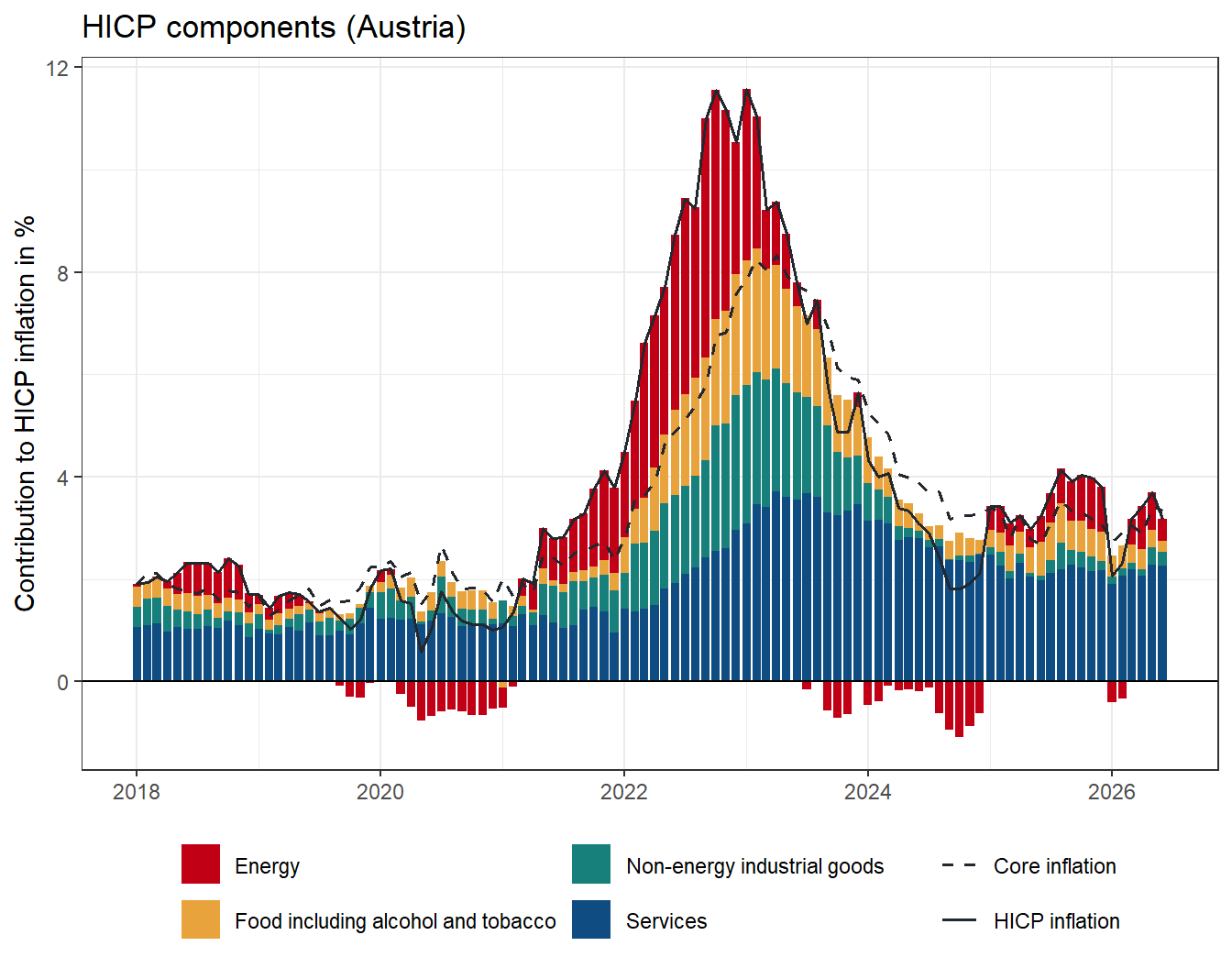
Headline inflation peaked at 11.6% in January 2023, higher and later than in the euro area. The contribution of services peaked at 3.7 percentage points in April 2023 and has barely come down since. In June 2026, with services prices 4.7% higher than a year earlier, services accounted for 2.3 of 3.2 points of headline inflation.
Services fell behind goods, and caught up
Chart 2 of the brief shows the price of services relative to goods as a four-quarter moving average with a log-linear trend fitted over 1996 to 2019 and extrapolated from there. The same chart for Austria, with the euro area series of the reproduction for comparison, uses quarterly averages of the unadjusted indices. The following function turns the monthly indices into quarterly averages, unadjusted for the chart and seasonally adjusted for the model below:
prepare_prices <- function(hicp) {

  monthly <- hicp %>%
    select(month, SERV, IGD_NNRG, GD) %>%
    pivot_longer(-month, names_to = "series", values_to = "index") %>%
    arrange(series, month) %>%

    # X-13ARIMA-SEATS with the defaults of seasonal, series by series
    group_by(series) %>%
    mutate(index_sa = ts(index, start = c(1996, 1), frequency = 12) %>%
             seas() %>%
             final() %>%
             as.numeric()) %>%
    ungroup()

  # Quarterly averages, dated by the start of the quarter: 1996.25 is 1996 Q2
  quarterly <- monthly %>%
    mutate(year = as.integer(substr(month, 1, 4)),
           month_of_year = as.integer(substr(month, 6, 7)),
           quarter = year + (month_of_year - 1) %/% 3 / 4) %>%
    group_by(series, quarter) %>%
    summarise(index = mean(index),
              index_sa = mean(index_sa),
              .groups = "drop")

  return(quarterly)
}

prices <- bind_rows(
  AT = prepare_prices(hicp),
  EA = prepare_prices(read.csv("../reproduction/_2026_hochmuth_petz_hicp.csv")),
  .id = "geo")
## Model used in SEATS is different: (0 2 1)(0 1 1)## Model used in SEATS is different: (2 2 2)(0 1 1)relative_prices <- prices %>%
select(geo, series, quarter, index) %>%
pivot_wider(names_from = series, values_from = index) %>%
pivot_longer(c(IGD_NNRG, GD),
names_to = "goods",
values_to = "goods_index") %>%
arrange(geo, goods, quarter) %>%
group_by(geo, goods) %>%
# Four-quarter moving average, indexed to Q1 2000 = 100
mutate(ratio = SERV / goods_index,
price = (ratio + lag(ratio) + lag(ratio, 2) + lag(ratio, 3)) / 4,
price = 100 * price / price[quarter == 2000]) %>%
# Log-linear trend fitted over 1996-2019, extrapolated from there
mutate(trend = exp(predict(lm(log(price) ~ quarter, subset = quarter < 2020),
newdata = data.frame(quarter = quarter))),
growth = 100 * coef(lm(log(price) ~ quarter,
subset = quarter < 2020))[["quarter"]]) %>%
ungroup()goods_labels <- c(IGD_NNRG = "Services relative to NEIG",
GD = "Services relative to overall goods")
relative_prices %>%
mutate(goods = factor(goods_labels[goods], levels = goods_labels)) %>%
pivot_longer(c(price, trend), names_to = "line", values_to = "value") %>%
ggplot(aes(x = quarter, y = value, colour = geo, linetype = line)) +
geom_hline(yintercept = 100) +
geom_line(linewidth = 0.8, na.rm = TRUE) +
facet_wrap(~ goods, ncol = 1, scales = "free_y") +
scale_colour_manual(values = c(AT = colours[["red"]],
EA = colours[["blue"]]),
labels = c(AT = "Austria", EA = "Euro area")) +
scale_linetype_manual(values = c(price = "solid", trend = "dashed"),
labels = c(price = "Relative price",
trend = "Trend 1996-2019")) +
labs(x = NULL,
y = "Relative price (Q1 2000 = 100)",
colour = NULL,
linetype = NULL) +
theme_bw() +
theme(legend.position = "bottom")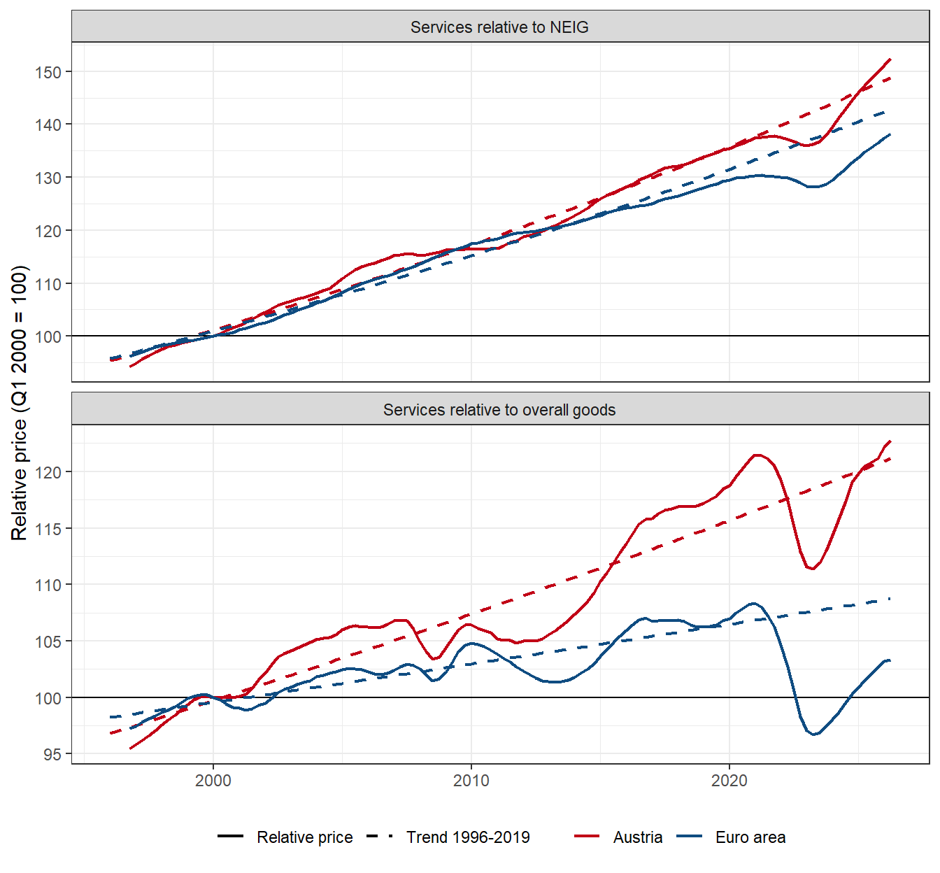
Before the pandemic, services in Austria became 1.5% a year more expensive relative to NEIG, against 1.3% in the euro area, and 0.7% relative to overall goods, against 0.3%. Up to 2021 the Austrian relative prices followed their trends closely, and in 2022 and 2023 they fell below them much like those of the euro area. The difference is what happened next. In the euro area the relative price of services is still 3.2% below its extrapolated trend against NEIG and 5% below it against overall goods in the second quarter of 2026. In Austria, services prices rose so much faster than goods prices from 2023 onwards that the relative price crossed its trend in 2025, and it is now 2.5% above it against NEIG and 1.3% above it against overall goods.
Estimation
Even though the catch-up seems to be over, the model is worth estimating, because it says how strongly Austrian prices respond to a gap at all. The estimation follows the reproduction. A function runs both stages for a country and either goods index: an OLS regression of the relative price on a trend over the whole sample, whose lagged residual enters create_bvarmodel as exogenous variable without further lags, s = 0. add_priors sets the paper’s priors, and the sampler is run for 5,000 burn-in draws, after which 20,000 are kept. The euro area is estimated again alongside Austria with the same code.
estimate_gap_model <- function(prices, other) {

  # Log prices of services (s) and of the other index (n), times 100
  y <- prices %>%
    filter(series %in% c("SERV", other)) %>%
    transmute(quarter,
              series = if_else(series == "SERV", "s", "n"),
              value = 100 * log(index_sa)) %>%
    pivot_wider(names_from = series, values_from = value) %>%
    arrange(quarter) %>%
    mutate(trend = row_number())

  # Stage 1: the relative-price gap is the residual of a linear trend
  stage_1 <- lm(s - n ~ trend, data = y)
  gap <- residuals(stage_1)

  # Stage 2: a VAR(1) in differences, with the lagged gap as exogenous
  # regressor
  dy <- ts(diff(as.matrix(y[, c("s", "n")])),
           start = y[["quarter"]][2],
           frequency = 4)

  ect <- ts(matrix(head(gap, -1), dimnames = list(NULL, "ect")),
            start = y[["quarter"]][2],
            frequency = 4)

  model <- create_bvarmodel(dy,
                            p = 1,
                            exogen = ect,
                            s = 0,
                            deterministic = "const",
                            iterations = 20000,
                            burnin = 5000)

  model <- add_priors(model,
                      coef = list(v_i = 1, v_i_det = 1),
                      sigma = list(df = 4, scale = 0.01))

  model <- add_initial_values(model, method = "ols")

  return(add_posterior_coefficients(model))
}

set.seed(20261012)

models <- list(AT_neig = estimate_gap_model(filter(prices, geo == "AT"),
                                            "IGD_NNRG"),
               AT_goods = estimate_gap_model(filter(prices, geo == "AT"), "GD"),
               EA_neig = estimate_gap_model(filter(prices, geo == "EA"),
                                            "IGD_NNRG"),
EA_goods = estimate_gap_model(filter(prices, geo == "EA"), "GD"))summary(models[["AT_neig"]])##
## Bayesian VAR model with p = 1 and s = 0
##
## Endogenous variables: s, n
##
## Variable: s
##
## Mean SD Naive SD Time-series SD 2.5% 50% 97.5%
## s.l1 0.77390 0.046440 3.284e-04 3.361e-04 0.68312 0.77345 0.865221 *
## n.l1 0.15321 0.038039 2.690e-04 2.690e-04 0.07937 0.15316 0.228735 *
## ect.l0 -0.01257 0.009643 6.819e-05 6.819e-05 -0.03152 -0.01249 0.006261
## const 0.11912 0.031244 2.209e-04 2.248e-04 0.05766 0.11932 0.180314 *
##
## Variable: n
##
## Mean SD Naive SD Time-series SD 2.5% 50% 97.5%
## s.l1 0.090338 0.09729 0.0006879 0.0006838 -0.09955 0.089699 0.28131
## n.l1 0.691794 0.07960 0.0005629 0.0005629 0.53448 0.692319 0.84477 *
## ect.l0 0.005535 0.02001 0.0001415 0.0001403 -0.03325 0.005614 0.04523
## const 0.026143 0.06568 0.0004644 0.0004660 -0.10246 0.026455 0.15464
##
## Variance-covariance matrix:
##
## Mean SD Naive SD Time-series SD 2.5% 50% 97.5%
## s_s 0.020179 0.002668 1.886e-05 1.958e-05 0.0156518 0.019946 0.02611 *
## s_n 0.008273 0.003993 2.823e-05 2.906e-05 0.0007924 0.008144 0.01652 *
## n_n 0.087522 0.011710 8.280e-05 8.639e-05 0.0674776 0.086407 0.11319 *The trend of the first stage is fitted over the whole sample including the recent years, so its gap differs from the one in the charts above, but it tells the same story. Against NEIG, the Austrian gap reached -4.5% in 2022 Q4 and is 3.9% in the second quarter of 2026, while the euro area gap went from -4.4% to 0.4%. Against overall goods, the Austrian gap is 1.9% and the euro area’s -1.4%.
The loadings of the four models, with 95% credible intervals:
loadings %>%
  kable(digits = 3,
        row.names = FALSE,
col.names = c("Model", "Loading", "Median", "2.5%", "97.5%"))| Model | Loading | Median | 2.5% | 97.5% |
|---|---|---|---|---|
| AT_neig | alpha_s | -0.012 | -0.032 | 0.006 |
| AT_neig | alpha_n | 0.006 | -0.033 | 0.045 |
| AT_goods | alpha_s | -0.004 | -0.016 | 0.007 |
| AT_goods | alpha_n | 0.054 | 0.001 | 0.106 |
| EA_neig | alpha_s | -0.033 | -0.054 | -0.012 |
| EA_neig | alpha_n | -0.010 | -0.038 | 0.017 |
| EA_goods | alpha_s | -0.030 | -0.045 | -0.015 |
| EA_goods | alpha_n | 0.057 | 0.010 | 0.105 |
In the euro area, services inflation responds clearly to a gap: \(\alpha_s\) is -0.033 with NEIG and -0.030 with overall goods, and both intervals exclude zero. In Austria the services loading is -0.012 with NEIG and -0.004 with goods, much smaller, and neither interval excludes zero. The direct response of Austrian services prices to where they stand relative to goods is weak. Goods prices respond in both places in the same way: with overall goods, \(\alpha_n\) is 0.054 in Austria and 0.057 in the euro area, so when services are cheap relative to goods, goods inflation slows.
How fast does the gap close?
The paper simulates the model in deviations from a baseline without a gap. From an initial gap \(z_0 = -1\), services about 1% cheaper relative to goods than their trend implies, and \(\Delta y_0 = 0\), the system evolves as
\[\Delta y_h = \alpha z_{h-1} + \Gamma \Delta y_{h-1}, \quad z_h = z_{h-1} + \Delta s_h - \Delta n_h,\]
and the cumulative contributions of services and goods inflation to closing it, in percent of the initial gap, are \(C_{s,h} = 100 \sum_{j \le h} \Delta s_j\) and \(C_{n,h} = -100 \sum_{j \le h} \Delta n_j\). The recursion is run for every posterior draw at once:
gap_closure <- function(model, horizon = 40) {

  # Equation i's coefficient on regressor j is in column (j - 1) k + i. The
  # regressors are the lags of s and n, the error correction term and the
  # constant
  draws <- as.matrix(model[["posterior"]][["a"]][["coeffs"]])
  k <- model[["model"]][["k"]]

  gamma_ss <- draws[, 1]
  gamma_ns <- draws[, 2]
  gamma_sn <- draws[, k + 1]
  gamma_nn <- draws[, k + 2]
  alpha_s <- draws[, 2 * k + 1]
  alpha_n <- draws[, 2 * k + 2]

  # Start from z_0 = -1 and dy_0 = 0
  n_draws <- nrow(draws)
  z <- rep(-1, n_draws)
  ds <- rep(0, n_draws)
  dn <- rep(0, n_draws)
  services <- rep(0, n_draws)
  other <- rep(0, n_draws)

  paths <- vector("list", horizon)

  for (h in seq_len(horizon)) {

    ds_new <- alpha_s * z + gamma_ss * ds + gamma_sn * dn
    dn_new <- alpha_n * z + gamma_ns * ds + gamma_nn * dn

    ds <- ds_new
    dn <- dn_new
    z <- z + ds - dn

    # Cumulative contributions, in % of the initial gap
    services <- services + 100 * ds
    other <- other - 100 * dn

    paths[[h]] <- data.frame(h = h,
                             remaining = -100 * z,
                             services = services,
                             other = other)
  }

  closure <- bind_rows(paths) %>%
    group_by(h) %>%
    summarise(lower = quantile(remaining, 0.16),
              upper = quantile(remaining, 0.84),
              remaining = median(remaining),
              services = median(services),
              other = median(other))

  start <- data.frame(h = 0,
                      lower = 100,
                      upper = 100,
                      remaining = 100,
                      services = 0,
                      other = 0)

  return(bind_rows(start, closure))
}

closure <- lapply(models, gap_closure) %>%
  bind_rows(.id = "model")
The chart shows the median of the remaining gap in Austria with its 68% credible interval, and the median contributions as bars that start at 100: bars pointing down close the gap, bars pointing up widen it. Where both contributions close the gap, they are stacked. The median remaining gap in the euro area is drawn for comparison.
closure <- closure %>%
  separate(model, c("region", "goods"), remove = FALSE) %>%
  mutate(goods = factor(goods, levels = c("neig", "goods"),
                        labels = c("Relative to NEIG",
                                   "Relative to overall goods")))

# Bars start at 100. Contributions with the same sign are stacked, opposite
# ones both start at 100
closure_bars <- closure %>%
  filter(region == "AT") %>%
  mutate(services_end = 100 - services,
         other_start = if_else(sign(other) == sign(services),
                               services_end,
                               100),
         other_end = other_start - other)

closure_bars <- bind_rows(
  transmute(closure_bars, h, goods, component = "Services",
            ymin = 100, ymax = services_end),
  transmute(closure_bars, h, goods,
            component = if_else(goods == "Relative to NEIG", "NEIG", "Goods"),
            ymin = other_start, ymax = other_end)) %>%
  mutate(component = factor(component, levels = c("Services", "NEIG", "Goods")))

ggplot(closure, aes(x = h)) +
  geom_rect(data = closure_bars,
            aes(xmin = h - 0.35, xmax = h + 0.35,
                ymin = pmin(ymin, ymax), ymax = pmax(ymin, ymax),
                fill = component),
            alpha = 0.45) +
  geom_ribbon(data = filter(closure, region == "AT"),
              aes(ymin = lower, ymax = upper),
              fill = colours[["ink"]],
              alpha = 0.2) +
  geom_hline(yintercept = c(0, 100)) +
  geom_line(aes(y = remaining, colour = region, linetype = region),
            linewidth = 0.9) +
  facet_wrap(~ goods, ncol = 1) +
  scale_fill_manual(values = c(Services = colours[["blue"]],
                               NEIG = colours[["teal"]],
                               Goods = colours[["amber"]])) +
  scale_colour_manual(values = c(AT = colours[["red"]],
                                 EA = colours[["ink"]]),
                      labels = c(AT = "Remaining gap, Austria",
                                 EA = "Remaining gap, euro area")) +
  scale_linetype_manual(values = c(AT = "solid", EA = "dashed"),
                        labels = c(AT = "Remaining gap, Austria",
                                   EA = "Remaining gap, euro area")) +
  labs(x = "Quarters after the initial gap",
       y = "% of initial gap",
       fill = NULL,
       colour = NULL,
       linetype = NULL,
       title = "What closes the gap? (Austria)") +
  theme_bw() +
  theme(legend.position = "bottom")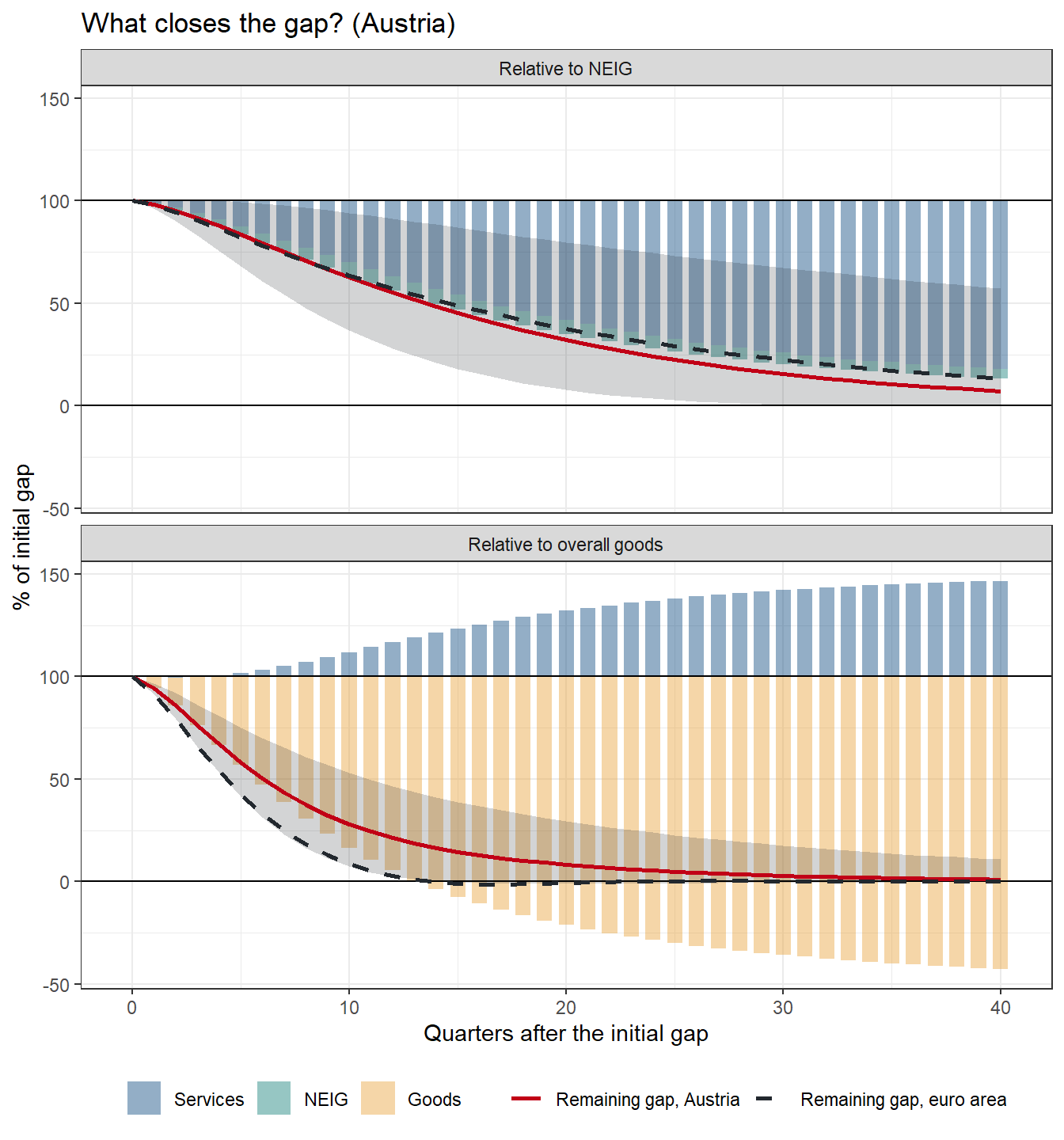
closure %>%
  filter(h %in% c(4, 8, 12, 20, 40)) %>%
  select(region, goods, h, remaining, services, other) %>%
  arrange(goods, region, h) %>%
  kable(digits = 0,
        row.names = FALSE,
        col.names = c("Region", "Goods index", "Quarter", "Remaining gap",
"Services", "Goods"))| Region | Goods index | Quarter | Remaining gap | Services | Goods |
|---|---|---|---|---|---|
| AT | Relative to NEIG | 4 | 88 | 9 | 3 |
| AT | Relative to NEIG | 8 | 71 | 23 | 6 |
| AT | Relative to NEIG | 12 | 55 | 37 | 7 |
| AT | Relative to NEIG | 20 | 32 | 58 | 7 |
| AT | Relative to NEIG | 40 | 7 | 82 | 5 |
| EA | Relative to NEIG | 4 | 86 | 21 | -7 |
| EA | Relative to NEIG | 8 | 71 | 46 | -17 |
| EA | Relative to NEIG | 12 | 57 | 68 | -26 |
| EA | Relative to NEIG | 20 | 38 | 101 | -40 |
| EA | Relative to NEIG | 40 | 13 | 142 | -57 |
| AT | Relative to overall goods | 4 | 67 | 0 | 33 |
| AT | Relative to overall goods | 8 | 37 | -7 | 69 |
| AT | Relative to overall goods | 12 | 21 | -17 | 95 |
| AT | Relative to overall goods | 20 | 8 | -32 | 121 |
| AT | Relative to overall goods | 40 | 1 | -47 | 143 |
| EA | Relative to overall goods | 4 | 54 | 14 | 32 |
| EA | Relative to overall goods | 8 | 18 | 21 | 61 |
| EA | Relative to overall goods | 12 | 3 | 23 | 74 |
| EA | Relative to overall goods | 20 | -1 | 22 | 80 |
| EA | Relative to overall goods | 40 | 0 | 21 | 79 |
Relative to NEIG, the gap closes about as fast in Austria as in the euro area: half of it is gone after 14 quarters, against 15. In both, services inflation does most of the work, but in different ways. In the euro area it responds strongly and has to make up for NEIG inflation, which works against the adjustment. In Austria the response of services inflation is weak but persistent – the coefficient of its own lag is above 0.7 – so it builds up over many quarters, and NEIG inflation does not work against it. Relative to overall goods, the Austrian gap is closed by goods inflation alone, while services inflation even works against it. Half of the gap is gone after 7 quarters, against 5 in the euro area.
A closer look at gastronomy
Austria is a tourism country, and it shows in its consumer basket. The HICP measures the spending of all households on the domestic territory, including that of foreign tourists, so restaurants, cafés and hotels weigh much more than in most other member states. Eurostat publishes indices and weights for food and beverage serving services, here called gastronomy, and accommodation services from 1996, and weights for services as a whole from 2000:
# Eurostat, ECOICOP ver. 2: services, gastronomy, accommodation and NEIG
gastronomy_filters <- list(geo = c("AT", "EA"),
                           unit = "I25",
                           coicop18 = c("SERV", "CP111", "CP112", "IGD_NNRG"))

get_eurostat("prc_hicp_minr",
             time_format = "raw",
             cache = FALSE,
             filters = gastronomy_filters) %>%
  transmute(geo,
            month = as.character(time),
            series = coicop18,
            index = values) %>%
  filter(month >= "2000-12", month <= "2026-06") %>%
  pivot_wider(names_from = series, values_from = index) %>%
  select(geo, month, SERV, CP111, CP112, IGD_NNRG) %>%
  arrange(geo, month) %>%
  write.csv("_2026-10-12-services-inflation-in-austria-gastronomy.csv",
            row.names = FALSE)

# Item weights in per mille of the total, available for services from 2000
gastronomy_weight_filters <- list(geo = c("AT", "EA"),
                                  coicop18 = c("SERV", "CP111", "CP112"))

get_eurostat("prc_hicp_iw",
             time_format = "raw",
             cache = FALSE,
             filters = gastronomy_weight_filters) %>%
  transmute(geo,
            year = as.integer(as.character(time)),
            series = coicop18,
            weight = values) %>%
  filter(year >= 2001, year <= 2026) %>%
  pivot_wider(names_from = series, values_from = weight) %>%
  select(geo, year, SERV, CP111, CP112) %>%
  arrange(geo, year) %>%
  write.csv("_2026-10-12-services-inflation-in-austria-gastronomy-weights.csv",
            row.names = FALSE)
gastronomy <- read.csv("_2026-10-12-services-inflation-in-austria-gastronomy.csv")
gastronomy_weights <- read.csv(
"_2026-10-12-services-inflation-in-austria-gastronomy-weights.csv")
# Weights as shares of services
shares <- gastronomy_weights %>%
transmute(geo, year, CP111 = CP111 / SERV, CP112 = CP112 / SERV)In 2026, gastronomy makes up 22% of the services in the Austrian basket and accommodation 10%, against 20% and 5% in the euro area. Together, they are about a third of Austrian services and a quarter of those of the euro area.
Contributions to services inflation
The contributions of the two items to services inflation follow from the same formula as above, with services as the aggregate and the weights as shares of services. Since the contributions of all services add up to services inflation, the remainder is the contribution of all other services:
services_contributions <- gastronomy %>%
  pivot_longer(c(CP111, CP112), names_to = "series", values_to = "index") %>%
  mutate(year = as.integer(substr(month, 1, 4))) %>%
  left_join(pivot_longer(shares, c(CP111, CP112),
                         names_to = "series", values_to = "weight"),
            by = c("geo", "year", "series")) %>%
  arrange(geo, series, month) %>%
  group_by(geo, series) %>%
  mutate(value = contribution(month, index, SERV, weight),
         rate = 100 * (SERV / lag(SERV, 12) - 1)) %>%
  ungroup() %>%
  filter(month >= "2018-01") %>%
  select(geo, month, series, value, rate) %>%
  pivot_wider(names_from = series, values_from = value) %>%
  mutate(OTHER = rate - CP111 - CP112,
         date = as.Date(paste0(month, "-01")))
services_colours <- c(CP111 = colours[["amber"]],
CP112 = colours[["teal"]],
OTHER = colours[["blue"]])
services_labels <- c(CP111 = "Gastronomy",
CP112 = "Accommodation",
OTHER = "Other services")
services_contributions %>%
pivot_longer(c(CP111, CP112, OTHER),
names_to = "component",
values_to = "value") %>%
mutate(component = factor(component, levels = names(services_colours)),
geo = factor(geo, levels = c("AT", "EA"),
labels = c("Austria", "Euro area"))) %>%
ggplot(aes(x = date, y = value)) +
geom_col(aes(fill = component), width = 25) +
geom_line(aes(y = rate, linetype = "Services inflation"),
linewidth = 0.7,
colour = colours[["ink"]]) +
geom_hline(yintercept = 0) +
facet_wrap(~ geo, ncol = 1) +
scale_fill_manual(values = services_colours, labels = services_labels) +
labs(x = NULL,
y = "Contribution to services inflation in %",
fill = NULL,
linetype = NULL,
title = "Services inflation and its components") +
theme_bw() +
theme(legend.position = "bottom")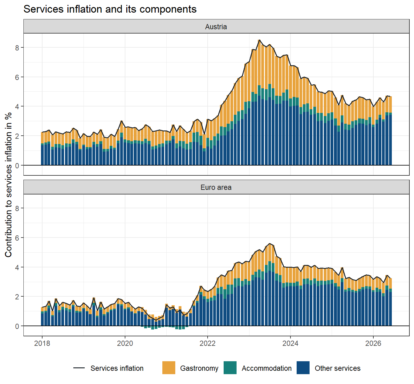
Gastronomy prices in Austria have risen by 52% since December 2019, against 31% in the euro area, while services as a whole became 34% and 24% more expensive. At its peak in April 2023, gastronomy alone contributed 3.1 of 8.5 percentage points of Austrian services inflation. In June 2026 it still contributes 1.1 of 4.7 points, against 0.7 of 3.2 in the euro area. Of the difference of 1.5 points between Austrian and euro area services inflation, gastronomy accounts for 0.4. The rest comes from other services, which are rising faster in Austria as well.
Services excluding gastronomy
Does gastronomy also explain why the relative price of services in Austria is above its trend? To find out, the price of services is split into gastronomy and the rest. Eurostat does not publish an index of services excluding gastronomy, but it can be derived from the chain-linking: within a year, the services index relative to December is the weighted average of its components relative to December, so the same holds for services without gastronomy with weights rescaled to add up to one,
\[\frac{P^{x}_t}{P^{x}_{D(y-1)}} = \frac{1}{1 - s_y} \left( \frac{P^s_t}{P^s_{D(y-1)}} - s_y \frac{P^g_t}{P^g_{D(y-1)}} \right),\]
where \(s_y\) is the share of gastronomy in services in year \(y\). Chaining these links from December 2000, the first December for which the weights of both are available, gives the index:
chain_excluding <- function(month, total, index, share) {
  year <- as.integer(substr(month, 1, 4))
  december <- match(paste0(year - 1, "-12"), month)
  link <- (total / total[december] - share * index / index[december]) /
    (1 - share)

  # The first month is a December, from which the links are chained
  result <- rep(100, length(month))
  for (t in seq_along(month)[-1]) {
    result[t] <- result[december[t]] * link[t]
  }

  return(result)
}

gastronomy <- gastronomy %>%
  mutate(year = as.integer(substr(month, 1, 4))) %>%
  left_join(select(shares, geo, year, share = CP111), by = c("geo", "year")) %>%
  arrange(geo, month) %>%
  group_by(geo) %>%
  mutate(SERV_X_CP111 = chain_excluding(month, SERV, CP111, share)) %>%
  ungroup()
The chart compares the price of the three relative to NEIG, as four-quarter moving averages of quarterly averages, indexed to 2019 = 100, with a log-linear trend fitted over 2001 to 2019:
series_labels <- c(SERV = "Services",
                   SERV_X_CP111 = "Services excluding gastronomy",
                   CP111 = "Gastronomy")

gastronomy_prices <- gastronomy %>%
  filter(month >= "2001-01") %>%
  mutate(quarter = year + (as.integer(substr(month, 6, 7)) - 1) %/% 3 / 4) %>%
  group_by(geo, quarter) %>%
  summarise(across(c(SERV, SERV_X_CP111, CP111, IGD_NNRG), mean),
            .groups = "drop") %>%
  pivot_longer(c(SERV, SERV_X_CP111, CP111),
               names_to = "series",
               values_to = "index") %>%
  arrange(geo, series, quarter) %>%
  group_by(geo, series) %>%

  # Four-quarter moving average, indexed to 2019 = 100
  mutate(ratio = index / IGD_NNRG,
         price = (ratio + lag(ratio) + lag(ratio, 2) + lag(ratio, 3)) / 4,
         price = 100 * price / mean(price[floor(quarter) == 2019])) %>%

  # Log-linear trend fitted over 2001-2019, extrapolated from there
  mutate(trend = exp(predict(lm(log(price) ~ quarter, subset = quarter < 2020),
                             newdata = data.frame(quarter = quarter))),
         growth = 100 * coef(lm(log(price) ~ quarter,
                                subset = quarter < 2020))[["quarter"]]) %>%
  ungroup() %>%
  mutate(series = factor(series_labels[series], levels = series_labels))
gastronomy_prices %>%
pivot_longer(c(price, trend), names_to = "line", values_to = "value") %>%
ggplot(aes(x = quarter, y = value, colour = geo, linetype = line)) +
geom_hline(yintercept = 100) +
geom_line(linewidth = 0.8, na.rm = TRUE) +
facet_wrap(~ series, ncol = 1, scales = "free_y") +
scale_colour_manual(values = c(AT = colours[["red"]],
EA = colours[["blue"]]),
labels = c(AT = "Austria", EA = "Euro area")) +
scale_linetype_manual(values = c(price = "solid", trend = "dashed"),
labels = c(price = "Relative price",
trend = "Trend 2001-2019")) +
labs(x = NULL,
y = "Price relative to NEIG (2019 = 100)",
colour = NULL,
linetype = NULL) +
theme_bw() +
theme(legend.position = "bottom")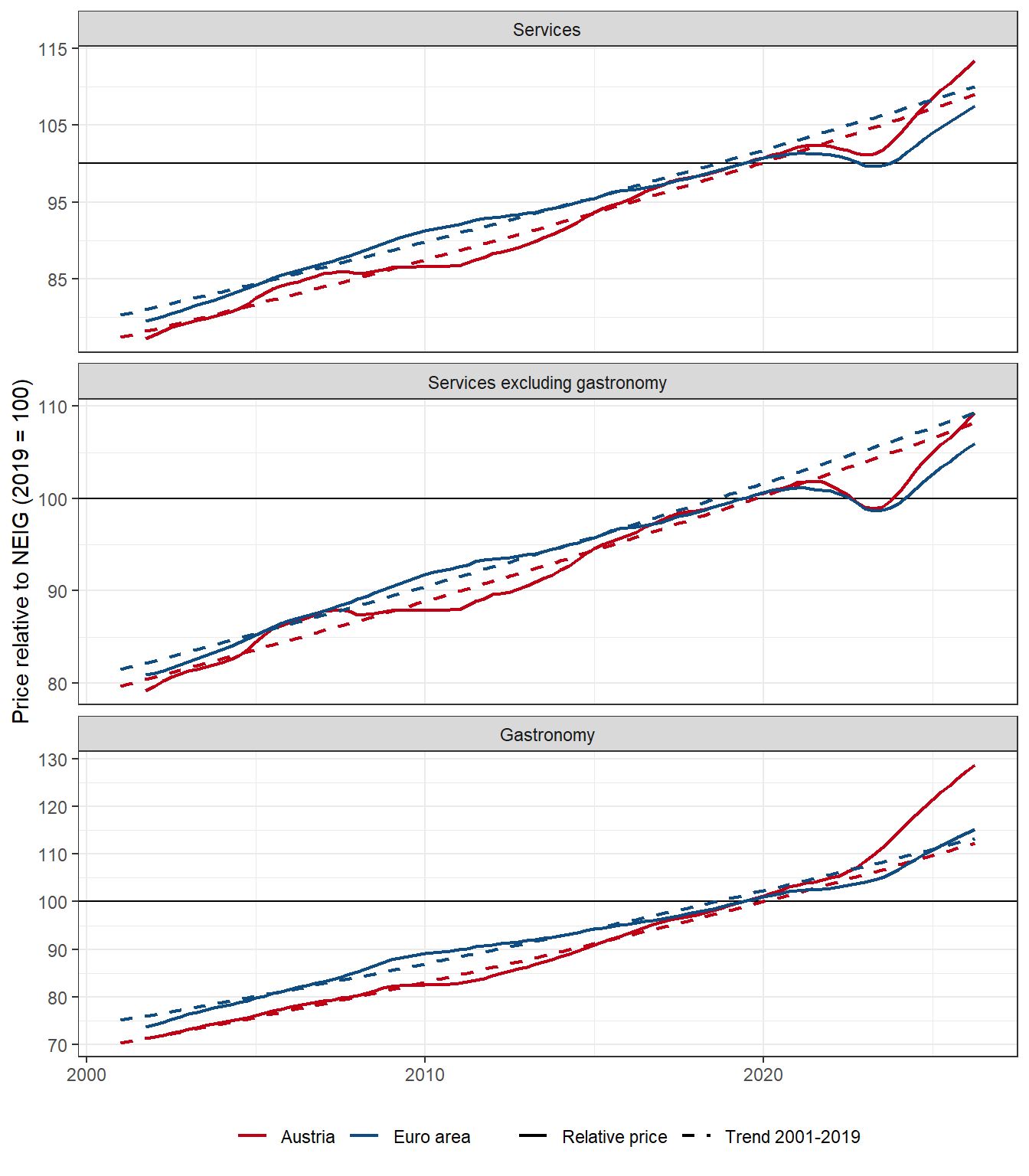
Gastronomy has been getting more expensive relative to NEIG for a long time, by 1.9% a year in Austria before the pandemic, against 1.6% in the euro area. Since 2022 the Austrian relative price has moved far away from that trend, and in the second quarter of 2026 it is 14.6% above it, while that of the euro area is within 1.7% of its trend. Without gastronomy, Austrian services are only 1% above their trend relative to NEIG, against 4% with it, and those of the euro area 3.1% below theirs. The figure for all services differs from the one in the first chart, because the trend is fitted from 2001 rather than 1996.
Gastronomy therefore explains most of the overshoot of the Austrian relative price. It does not explain why services inflation is still high, though: without gastronomy, Austrian services prices are 4.6% higher than a year earlier, almost as much as with it, and well above the 3.1% of the euro area.
What it means
Hochmuth and Petz argue that services inflation in the euro area stays high partly because the price of services has to catch up with that of goods after the shock of 2021 and 2022. For Austria, the data tell a different story:
- The catch-up is over. The relative price of services fell below its trend in Austria about as much as in the euro area, but it has since climbed back above it, against NEIG and against overall goods. Whatever keeps Austrian services inflation above 4% today, it is not a gap that still has to be closed.
- Gastronomy is behind the overshoot, but not behind today’s inflation. Restaurants and cafés weigh much more in Austria than in the euro area, their prices have risen by half since 2019 and they are far above their long-run trend relative to goods. Without them, the relative price of Austrian services is close to its trend. Today’s services inflation, however, is broad: services excluding gastronomy rise almost as fast.
- If anything, the gap now argues for lower services inflation. The model is symmetric: with services above their trend relative to goods, it expects services inflation to slow and goods inflation to pick up. The direct response of Austrian services prices is weak and uncertain, though, so this pull is slow, and relative to overall goods it was goods prices that did the adjusting in the past.
- Other explanations are needed. Candidates specific to Austria are wage settlements that take the inflation of the past year as their starting point, which pass the energy shock on to labour-intensive services such as gastronomy with a delay, strong demand from tourism, and the indexation of rents and many administered prices to past inflation. Testing them is beyond the scope of a model with two prices.
There are also reasons for caution. A straight line fitted to thirty years of data is sensitive to its end points, and the finding that Austria is above its trend depends on the trend not having steepened. And the gap is the residual of a first stage whose uncertainty is not carried over to the second, a simplification of the paper that this post keeps.
A follow-up post estimates the model for all 21 countries of the euro area.
References
Engle, R. F., & Granger, C. W. J. (1987). Co-integration and error correction: Representation, estimation, and testing. Econometrica, 55(2), 251–276. https://doi.org/10.2307/1913236
Hochmuth, P., & Petz, N. (2026). On the persistence of services inflation and the price of services relative to goods. OeNB Policy Brief 2026/11. Oesterreichische Nationalbank. https://www.oenb.at/en/daten-und-forschung/publikationen/publikationsreihen/policy-brief/2026/policy-brief-2026-11.html
Ribe, M. (1999). Effects of subcomponents on chained price indices like the HICPs and the MUICP. Statistics Sweden.
Sax, C., & Eddelbuettel, D. (2018). Seasonal adjustment by X-13ARIMA-SEATS in R. Journal of Statistical Software, 87(11), 1–17. https://doi.org/10.18637/jss.v087.i11
