An Introduction to Factor-Augmented Vector Autoregression (FAVAR)
with tags r var favar factor-model bvartools monetary-policy impulse-responseIntroduction
As we saw in the post on vector autoregressive (VAR) models, traditional VAR models suffer from a so-called curse of dimensionality. Each additional variable adds a further equation and a further lag polynomial to every other equation, so the number of coefficients grows with the square of the number of variables. With the few decades of quarterly data that are usually available this limits a VAR to a handful of variables. Policy makers, however, base their decisions on a much larger set of indicators than a VAR can accommodate, and leaving that information out of the model can distort the results.
Factor-augmented VAR (FAVAR) models address this issue. They summarise the information in a large panel of time series by a small number of factors, which are common drivers of the observed variables, and add these factors to an otherwise standard VAR. The idea behind factors becomes clear when looking at a few measures of economic activity. Growth in GDP, industrial production and private consumption measure different things, but they move together:
library("bvartools")
library("ggplot2")
library("scales")
library("tidyr")

# Download a fixed vintage of the FRED-QD database
qd_url <- paste0("https://www.stlouisfed.org/-/media/project/frbstl/",
                 "stlouisfed/research/fred-md/quarterly/2026-09-qd.csv")
qd_raw <- read.csv(qd_url)

# The first two rows contain information on the series, the rest the data
flag <- unlist(qd_raw[1, -1])
tcode <- unlist(qd_raw[2, -1])
dates <- as.Date(qd_raw[-(1:2), 1], format = "%m/%d/%Y")
qd_levels <- as.matrix(qd_raw[-(1:2), -1])

# Sample period
in_sample <- dates >= as.Date("1960-01-01") & dates <= as.Date("2007-12-01")

# Year-on-year growth of three measures of economic activity
activity <- c(GDPC1 = "GDP",
              INDPRO = "Industrial production",
              PCECC96 = "Private consumption")
growth <- apply(log(qd_levels[, names(activity)]),
                2,
                function(x) {return(c(rep(NA, 4), diff(x, lag = 4)))})
colnames(growth) <- activity

temp <- data.frame(date = dates, growth, check.names = FALSE)[in_sample, ]
temp <- pivot_longer(temp, cols = -date)

ggplot(temp, aes(x = date, y = value, colour = name)) +
  geom_hline(yintercept = 0) +
  geom_line() +
  scale_y_continuous(labels = percent_format()) +
  theme_bw() +
  theme(legend.position = "bottom",
        legend.title = element_blank()) +
  labs(title = "Measures of economic activity",
       x = NULL,
       y = "Log-growth rate (y-o-y)",
       caption = "Source: FRED-QD, vintage 2026-09.")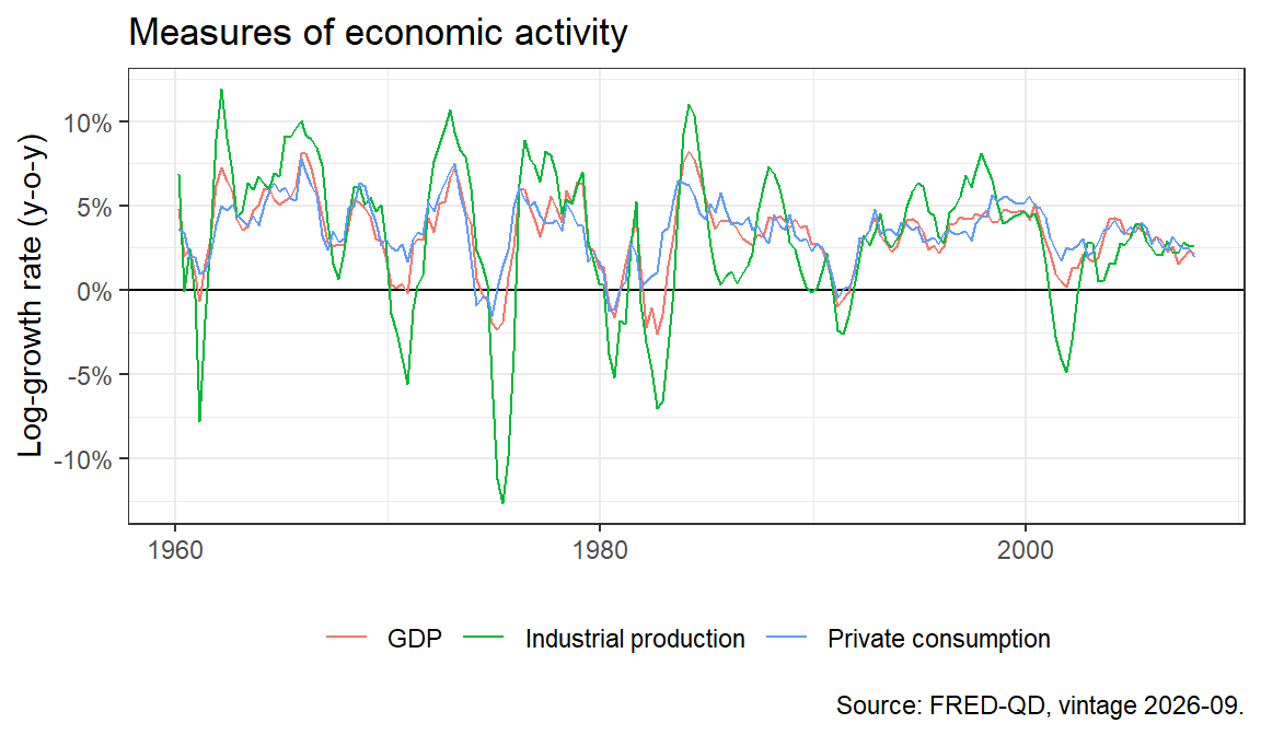
Although each indicator measures a different economic phenomenon, they follow a common pattern. This pattern can be understood as an unobserved process, which drives the observed indicators and which could be labelled economic activity. Estimating such processes is the job of a dynamic factor model, and Stock and Watson (2002) showed that a few factors from a large panel of series are useful for forecasting. A FAVAR goes one step further and lets the factors interact with observed variables of interest in a VAR.
The model
Following Bernanke, Boivin and Eliasz (2005), BBE hereafter, a FAVAR model consists of two equations. The transition equation1 describes the dynamic relationship between a \(K \times 1\) vector of observed variables \(y_t\) and an \(N \times 1\) vector of unobserved factors \(f_t\):
\[ \begin{bmatrix} f_{t} \\ y_{t} \end{bmatrix} = c + A_{1} \begin{bmatrix} f_{t-1} \\ y_{t-1} \end{bmatrix} + \dots + A_p \begin{bmatrix} f_{t-p} \\ y_{t-p} \end{bmatrix} + u_t,\]
where \(A_1, \dots, A_p\) are coefficient matrices, \(c\) is a vector of intercepts and \(u_t \sim N(0, \Sigma_u)\). Apart from the fact that some of its variables are unobserved, this is an ordinary VAR model. Hence the name factor-augmented vector autoregression.
The measurement equation links the factors to a large \(M \times 1\) vector of observed series \(x_t\), which is often called the informational panel:
\[ x_t = \lambda^{f} f_t + \lambda^{y} y_t + \epsilon_t,\]
where \(\lambda^{f}\) is the matrix of factor loadings and \(\epsilon_t\) is an error term with mean zero, whose covariance matrix is usually assumed to be diagonal. \(y_t\) enters the equation as well, so that \(x_t\) can react to the observed variables directly and the factors only capture the information that is not already contained in \(y_t\). \(M\) can be much larger than the number of observations, while \(N\) is small.
Since the factors are unobserved, they are only identified up to a rotation: multiplying \(f_t\) by an invertible matrix and the loadings by its inverse leaves the measurement equation unchanged. Each estimation method therefore needs a normalisation. In a Bayesian estimation of the whole system this is commonly achieved by restricting a block of \(\lambda^{f}\). The two-step approach below uses principal components, which are identified by the normalisation that the factors are orthogonal.
Two-step estimation
BBE propose two methods for the estimation of a FAVAR. One is a Bayesian approach, which samples the factors and the parameters of both equations jointly. The other is a simple two-step procedure:
- Estimate the space spanned by \(f_t\) and \(y_t\) by the principal components of \(x_t\).
- Estimate the transition equation as a VAR, in which the factors from the first step are treated as if they were observed.
The application below uses the two-step procedure first and compares it with the one-step approach at the end.
There is a catch in the first step. The principal components of the whole panel also contain the information of \(y_t\), since the panel includes many series that respond to it. BBE’s application is the effect of monetary policy, where \(y_t\) is the federal funds rate. As in many VAR studies of monetary policy, a recursive identification scheme is used, which assumes that the policy rate reacts to economic conditions within a period, while the economy reacts to a policy shock with a lag. This requires factors that do not respond to the policy rate in the same period, which the principal components of the whole panel do not satisfy.
BBE solve this by splitting the panel into slow-moving variables, like output, employment and prices, which are assumed not to react to monetary policy within the same period, and fast-moving variables, like asset prices and interest rates, which are allowed to react immediately. The principal components of the slow-moving variables do not depend on the policy rate in the same period by construction. They are used to clean the factors of the whole panel from the direct effect of the policy rate: the factors are regressed on the slow-moving factors and the policy rate, and the part that is explained by the policy rate is removed.
Application
The following application estimates the effect of a monetary policy shock on the US economy in the spirit of BBE. They used monthly data up to 2001. Here, the quarterly FRED-QD database of McCracken and Ng (2020) is used, which contains about 250 macroeconomic time series and is updated every month. One vintage is pinned in the code above, so that the results can be reproduced. The sample runs from 1960Q1 to 2007Q4, so that the zero lower bound period, in which the federal funds rate stopped being the main instrument of monetary policy, is excluded.
Data
The first row of the FRED-QD file marks the series that McCracken and Ng (2020) use for factor estimation. These exclude aggregates of other series in the database to avoid double counting. The second row contains a code for the transformation that makes a series stationary. Most of them are first differences or log differences. For prices the database suggests second differences of logs. Since this would treat inflation as non-stationary, which is not what BBE do, prices are used as log differences here, i.e. as inflation rates.
# Transformations, which are applied to the series
transform_series <- function(x, code) {
  result <- switch(as.character(code),
                   "1" = x,                   # Level
                   "2" = c(NA, diff(x)),      # First difference
                   "4" = log(x),              # Log level
                   "5" = c(NA, diff(log(x))), # Log difference
                   # Log difference instead of second difference
                   "6" = c(NA, diff(log(x))),
                   rep(NA, length(x)))        # Codes that are not used here
  return(result)
}

# Transform all series and select the sample period
x <- sapply(colnames(qd_levels),
            function(i) {return(transform_series(qd_levels[, i], tcode[i]))})
x <- x[in_sample, ]

# Federal funds rate in levels
ffr <- qd_levels[in_sample, "FEDFUNDS"]

# Informational panel: series for factor estimation without missing values
panel <- names(flag)[flag == 1 & names(flag) != "FEDFUNDS"]
panel <- panel[colSums(is.na(x[, panel])) == 0]
x_panel <- scale(x[, panel])
This leaves an informational panel of 100 series with 192 observations each, which are standardised to have mean zero and unit variance, so that no series dominates the principal components because of its scale.
FRED-QD sorts its series into groups. The slow-moving variables are taken from the groups on national accounts, industrial production, employment and unemployment, prices, as well as earnings and productivity. The remaining groups, which contain housing, orders, interest rates, money and credit, household balance sheets, exchange rates and stock prices, are treated as fast-moving.
# Names of the series between two series in the database
series_range <- function(from, to) {
  series <- colnames(qd_levels)
  return(series[match(from, series):match(to, series)])
}

slow <- intersect(panel, c(series_range("GDPC1", "HWIx"),
                           series_range("PCECTPI", "UNLPNBS")))
Factors
The number of factors is a choice of the researcher. BBE report results for different numbers of factors, and three is a common choice in their paper, which is used here as well.
n_factors <- 3

# Principal components of the whole panel and of the slow-moving variables
pc_all <- prcomp(x_panel)
f_all <- pc_all[["x"]][, 1:n_factors]
f_slow <- prcomp(x_panel[, slow])[["x"]][, 1:n_factors]

# Remove the direct effect of the federal funds rate
fit <- lm(f_all ~ f_slow + ffr)
f <- f_all - outer(ffr, coef(fit)["ffr", ])
colnames(f) <- paste0("f", 1:n_factors)

# Share of the variance of the panel explained by each factor
share <- summary(pc_all)[["importance"]][2, 1:n_factors]
The three factors explain 20, 14 and 7 per cent of the variance of the panel. These are substantial shares for a panel that combines real activity, prices, financial markets and survey data.
The transition equation
The cleaned factors and the federal funds rate form the vector of variables in the transition equation. It is estimated as a Bayesian VAR with four lags and a constant using the bvartools package. The priors on the coefficients and the error covariance are weakly informative.
y <- ts(cbind(f, ffr = ffr), start = c(1960, 1), frequency = 4)

set.seed(20261012)
model <- create_bvarmodel(y,
                          p = 4,
                          deterministic = "const",
                          iterations = 10000,
                          burnin = 2000)
model <- add_priors(model,
                    coef = list(v_i = 1 / 10, v_i_det = 1 / 100),
                    sigma = list(df = 6, scale = 1))
model <- add_initial_values(model)
model <- add_posterior_coefficients(model)
The monetary policy shock is identified recursively by ordering the federal funds rate last. Thus, the factors do not react to the shock in the quarter in which it occurs, while the federal funds rate can react to all factors within the same quarter. This corresponds to the orthogonalised impulse response, which is calculated by the irf function. The draws of the responses are kept, because they are needed to compute the responses of the series in the panel below. Each draw is rescaled, so that the shock raises the federal funds rate by 25 basis points on impact.
responses <- lapply(colnames(y), function(i) {
  result <- irf(model,
                impulse = "ffr",
                response = i,
                n_ahead = 20,
                type = "oir",
                keep_draws = TRUE)
  return(unclass(result))
})
names(responses) <- colnames(y)

# Rescale each draw to a shock of 25 basis points
shock_scale <- 0.25 / responses[["ffr"]][, 1]
responses <- lapply(responses, function(r) {return(r * shock_scale)})
Responses of observed series
The main advantage of a FAVAR is that the responses of every series in the database can be obtained from the responses of the factors and the federal funds rate. This is what the measurement equation is for: the loadings of a series are estimated by a regression on the factors and the federal funds rate, and its impulse response is the corresponding weighted sum of the responses in the transition equation. The series do not need to be part of the panel, from which the factors are extracted. Real GDP, for example, is an aggregate and therefore excluded from the panel, but its response can still be calculated.
Since the series enter the model as differences, their responses are cumulated to obtain the response of their levels. Responses of series in logs are multiplied by 100, so that they are percentage deviations.
show_series <- c(GDPC1 = "Real GDP",
                 INDPRO = "Industrial production",
                 PAYEMS = "Payroll employment",
                 UNRATE = "Unemployment rate",
                 CPIAUCSL = "Consumer prices",
                 HOUST = "Housing starts",
                 M2REAL = "Real M2",
                 S.P.500 = "S&P 500")

# Loadings of the series on the factors and the federal funds rate
x_loadings <- coef(lm(x[, names(show_series)] ~ unclass(y)))[-1, ]

# Responses of the series, cumulated to levels
ir_x <- lapply(names(show_series), function(i) {
  weighted <- Map(function(ir, l) {return(ir * l)},
                  responses,
                  x_loadings[, i])
  r <- Reduce(`+`, weighted)
  r <- t(apply(r, 1, cumsum))
  if (tcode[i] != 2) {
    r <- 100 * r
  }
  return(r)
})
names(ir_x) <- names(show_series)
ir_x[["FEDFUNDS"]] <- responses[["ffr"]]

# Median and 90 per cent credible intervals
unit_labels <- c(show_series, FEDFUNDS = "Federal funds rate")
in_pp <- names(unit_labels) %in% c("UNRATE", "FEDFUNDS")
unit_labels <- paste0(unit_labels, ifelse(in_pp, " (pp)", " (%)"))
names(unit_labels) <- c(names(show_series), "FEDFUNDS")
panel_order <- unit_labels[c("FEDFUNDS", names(show_series))]

summarise_irf <- function(r, name) {
  q <- apply(r, 2, quantile, probs = c(0.05, 0.5, 0.95))
  result <- data.frame(variable = name,
                       h = 0:(ncol(r) - 1),
                       lower = q[1, ],
                       median = q[2, ],
                       upper = q[3, ])
  return(result)
}
temp <- do.call(rbind, Map(summarise_irf, ir_x, unit_labels[names(ir_x)]))
temp[["variable"]] <- factor(temp[["variable"]], levels = panel_order)
ggplot(temp, aes(x = h, y = median)) +
geom_hline(yintercept = 0, colour = "grey50") +
geom_ribbon(aes(ymin = lower, ymax = upper),
fill = "steelblue",
alpha = 0.3) +
geom_line(colour = "steelblue4") +
facet_wrap(~ variable, scales = "free_y", ncol = 3) +
theme_bw() +
labs(title = "Responses to a monetary policy shock of 25 basis points",
x = "Quarters",
y = NULL,
caption = "Median and 90 per cent credible intervals.")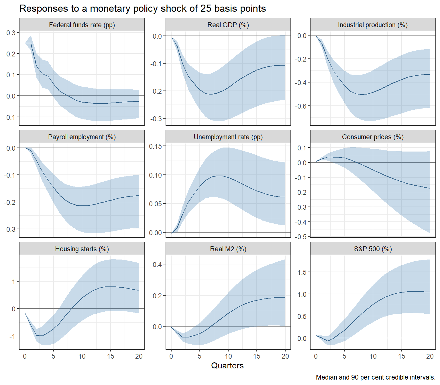
The responses look like what economic theory predicts. After the initial increase the federal funds rate returns to its previous level within about two years. Real activity declines with a lag: real GDP falls by up to 0.21 per cent after 7 quarters and industrial production by up to 0.5 per cent. Payroll employment falls as well and the unemployment rate rises by up to 0.1 percentage points. Housing starts, which are known to be sensitive to interest rates, react quickly and strongly, but recover after about two years and even overshoot. The response of the S&P 500 is less plausible, since stock prices rise after about two years. This is one of the cases, where the responses of individual series should be interpreted with caution, since they depend on how well the few factors capture the series’ dynamics.
The response of consumer prices deserves a closer look. They rise slightly during the first year and decline afterwards. After five years, the price level is 0.17 per cent lower than without the shock, although the credible interval still includes zero.
The price puzzle
The response of prices is one of the main motivations behind the FAVAR approach. Small VAR models of monetary policy frequently find that prices rise after a monetary tightening, which is known as the price puzzle (Sims, 1992). A common explanation is that the central bank reacts to information about future inflation, which a small VAR does not contain. A tightening then looks like the cause of the subsequent inflation, which it actually tried to prevent. Adding factors from a large panel provides the model with much of the information that the central bank has at its disposal.
To illustrate this, the same recursive identification is applied to a small VAR with GDP growth, inflation and the federal funds rate.
small <- cbind(gdp = 100 * x[, "GDPC1"],
               cpi = 100 * x[, "CPIAUCSL"],
               ffr = ffr)
small <- ts(small, start = c(1960, 1), frequency = 4)

small_model <- create_bvarmodel(small,
                                p = 4,
                                deterministic = "const",
                                iterations = 10000,
                                burnin = 2000)
small_model <- add_priors(small_model,
                          coef = list(v_i = 1 / 10, v_i_det = 1 / 100),
                          sigma = list(df = 6, scale = 1))
small_model <- add_initial_values(small_model)
small_model <- add_posterior_coefficients(small_model)

# Responses of inflation and the federal funds rate
small_cpi <- irf(small_model,
                 impulse = "ffr",
                 response = "cpi",
                 n_ahead = 20,
                 type = "oir",
                 keep_draws = TRUE)
small_cpi <- unclass(small_cpi)
small_ffr <- irf(small_model,
                 impulse = "ffr",
                 response = "ffr",
                 n_ahead = 0,
                 type = "oir",
                 keep_draws = TRUE)
small_ffr <- unclass(small_ffr)

# Rescale to 25 basis points and cumulate inflation to the price level
small_cpi <- t(apply(small_cpi * 0.25 / small_ffr[, 1], 1, cumsum))
temp <- rbind(summarise_irf(small_cpi, "VAR"),
summarise_irf(ir_x[["CPIAUCSL"]], "FAVAR"))
ggplot(temp, aes(x = h, y = median, colour = variable, fill = variable)) +
geom_hline(yintercept = 0, colour = "grey50") +
geom_ribbon(aes(ymin = lower, ymax = upper), alpha = 0.2, colour = NA) +
geom_line() +
theme_bw() +
theme(legend.position = "bottom",
legend.title = element_blank()) +
labs(title = "Response of consumer prices (%)",
x = "Quarters",
y = NULL,
caption = "Median and 90 per cent credible intervals.")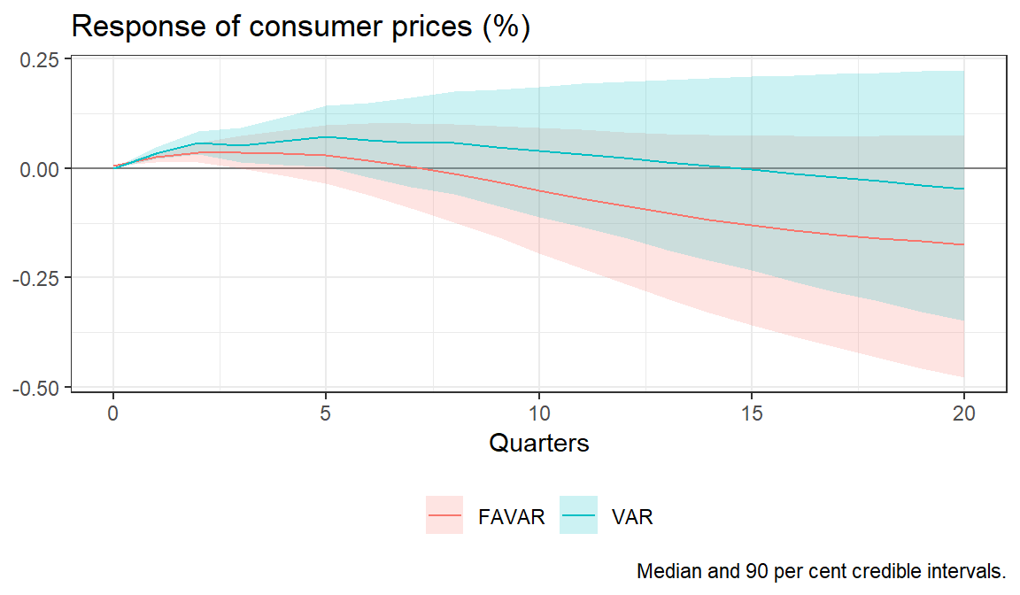
Both models show an increase of the price level after the tightening. In the small VAR it is larger and more persistent: after four quarters the median response is 0.06 per cent compared to 0.03 per cent in the FAVAR, and the median falls below zero only after 15 quarters, while in the FAVAR it does so after 8 quarters. The additional information in the factors therefore weakens the price puzzle, although it does not remove it completely. BBE report a similar result for their sample.
One-step estimation
The two-step approach is simple and fast, but it has a drawback. The factors are estimates, which are treated as if they were observed in the second step. The credible intervals above therefore do not account for the uncertainty about the factors. BBE address this by a bootstrap procedure and by their Bayesian one-step approach, which draws the factors together with the other parameters of the model, so that the uncertainty about the factors enters the credible intervals. They find that both approaches lead to qualitatively similar results.
The one-step approach is implemented in the dfmtools package, whose installation is described in the post on dynamic factor models. Its Gibbs sampler draws the factors, the loadings, the coefficients of the transition equation and the covariance matrices of both error terms in turn.
Since the factors are no longer principal components, they need a different normalisation. dfmtools restricts the leading \(N \times N\) block of \(\lambda^{f}\) to the identity matrix and the corresponding rows of \(\lambda^{y}\) to zero. Thus, the first \(N\) series of the panel are the factors plus idiosyncratic noise. This makes the order of the panel a substantive choice: the first series should be broad slow-moving measures, since they define the factors. Following the vignette of the package, industrial production, payroll employment and consumer prices are used. They are aggregates and not part of the panel above, so they are added at the beginning. The same is done for the remaining series, whose responses are shown below, since the one-step approach only produces responses for the series of the panel.
library("dfmtools")

# Series that define the factors and further series, whose responses are shown
identifiers <- c("INDPRO", "PAYEMS", "CPIAUCSL")
extra <- c("GDPC1", "UNRATE", "HOUST", "M2REAL")
panel_one <- c(identifiers, extra, setdiff(panel, c(identifiers, extra)))

x_one <- ts(x[, panel_one], start = c(1960, 1), frequency = 4)
ffr_one <- ts(cbind(FEDFUNDS = ffr), start = c(1960, 1), frequency = 4)

# Slow-moving series
slow_one <- c(identifiers, "GDPC1", "UNRATE", slow)
Instead of cleaning the factors, the distinction between slow-moving and fast-moving variables enters the model as a restriction: the loadings of the slow-moving series on the federal funds rate are set to zero, so that they cannot react to it within the same quarter. Together with the identity block this implies that the factors do not react to the policy rate within the quarter either. The restriction is specified with argument slow of add_priors. The model has the same number of factors and lags as above, and create_favarmodel normalises the series of the panel by default.
favar <- create_favarmodel(x = x_one,
                           y = ffr_one,
                           p = 4,
                           n = 3,
                           iterations = 10000,
                           burnin = 2000)
favar <- add_priors(favar, slow = slow_one)
favar <- add_initial_values(favar)
favar <- add_posterior_coefficients(favar)
The restriction is implemented as a very tight prior rather than as an exact zero, but the posterior means of the restricted loadings are zero to 7 decimal places, which is exact for all practical purposes.
The irf method of dfmtools computes the responses of the series in the panel directly from the loadings. As before, the shock is identified recursively with the federal funds rate ordered last and each draw is rescaled to a shock of 25 basis points. Since the panel is normalised, the responses are multiplied by the standard deviation of the respective series to obtain them in their original units.
# Response of the federal funds rate, used to rescale the shock
ffr_draws <- irf(favar,
                 impulse = "FEDFUNDS",
                 response = "FEDFUNDS",
                 n_ahead = 20,
                 keep_draws = TRUE)
ffr_draws <- unclass(ffr_draws)
one_scale <- 0.25 / ffr_draws[, 1]
x_scale <- attr(favar[["data"]][["x"]], "scaled:scale")

ir_one <- lapply(names(show_series), function(i) {
  r <- irf(favar,
           impulse = "FEDFUNDS",
           response = i,
           n_ahead = 20,
           cumulative = TRUE,
           keep_draws = TRUE)
  r <- unclass(r)
  r <- r * one_scale * x_scale[i]
  if (tcode[i] != 2) {
    r <- 100 * r
  }
  return(r)
})
names(ir_one) <- names(show_series)
ir_one[["FEDFUNDS"]] <- ffr_draws * one_scale
two_step <- Map(summarise_irf, ir_x, unit_labels[names(ir_x)])
two_step <- cbind(do.call(rbind, two_step), method = "Two-step")
one_step <- Map(summarise_irf, ir_one, unit_labels[names(ir_one)])
one_step <- cbind(do.call(rbind, one_step), method = "One-step")
temp <- rbind(two_step, one_step)
temp[["variable"]] <- factor(temp[["variable"]], levels = panel_order)
ggplot(temp, aes(x = h, y = median, colour = method, fill = method)) +
geom_hline(yintercept = 0, colour = "grey50") +
geom_ribbon(aes(ymin = lower, ymax = upper), alpha = 0.2, colour = NA) +
geom_line() +
facet_wrap(~ variable, scales = "free_y", ncol = 3) +
theme_bw() +
theme(legend.position = "bottom",
legend.title = element_blank()) +
labs(title = "Responses to a monetary policy shock of 25 basis points",
x = "Quarters",
y = NULL,
caption = "Median and 90 per cent credible intervals.")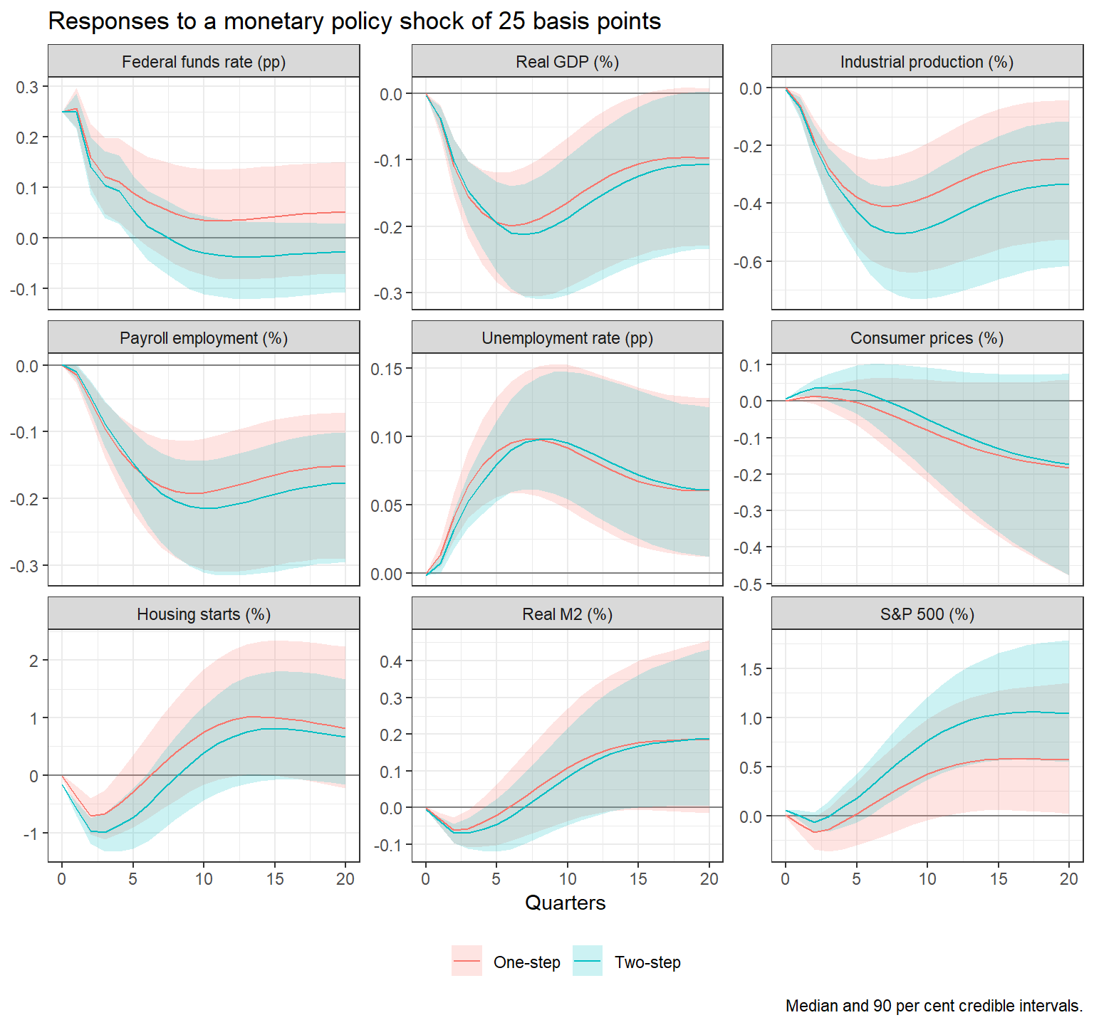
Both approaches tell the same story. In the one-step model, real GDP falls by up to 0.2 per cent after 6 quarters, compared to 0.21 per cent after 7 quarters in the two-step model, and the other real variables and prices respond very similarly as well. The federal funds rate is somewhat more persistent in the one-step model. The initial increase of consumer prices almost disappears, and the less plausible rise of the S&P 500 is about half as large as in the two-step model. The width of the credible intervals of the series in the panel is between 1.0 and 1.3 times that of the two-step approach. Thus, accounting for the uncertainty about the factors does not change the conclusions in this application.
Remarks
A FAVAR, whose loadings and coefficients vary over time, is used by Koop and Korobilis (2014) to construct an index of financial conditions. Their approach is reproduced here.
References
Bernanke, B. S., Boivin, J., & Eliasz, P. (2005). Measuring the effects of monetary policy: A factor-augmented vector autoregressive (FAVAR) approach. The Quarterly Journal of Economics, 120(1), 387-422. https://doi.org/10.1162/0033553053327452
Koop, G., & Korobilis, D. (2014). A new index of financial conditions. European Economic Review, 71, 101-116. https://doi.org/10.1016/j.euroecorev.2014.07.002
McCracken, M. W., & Ng, S. (2020). FRED-QD: A quarterly database for macroeconomic research. NBER Working Paper 26872. https://doi.org/10.3386/w26872
Sims, C. A. (1992). Interpreting the macroeconomic time series facts: The effects of monetary policy. European Economic Review, 36(5), 975-1000. https://doi.org/10.1016/0014-2921(92)90041-T
Stock, J. H., & Watson, M. W. (2002). Macroeconomic forecasting using diffusion indexes. Journal of Business & Economic Statistics, 20(2), 147-162. https://doi.org/10.1198/073500102317351921
The terms measurement and transition equation stem from the close relationship of the FAVAR approach to state space models.↩︎
