An Introduction to Stationarity and Unit Roots in Time Series Analysis
with tags r stationarity unit-root cointegration time-series -Concepts
Basically stationarity means that a time series has a constant mean and constant variance over time. Althouth not particularly imporant for the estimation of parameters of econometric models these features are essential for the calculation of reliable test statistics and, hence, can have a significant impact on model selection.
To illustrate this concept, let’s look at quarterly data on disposable income in billion DM from 1960 to 1982, which is data set E1 from Luetkepohl (2007).
# Load data
library(bvartools)
data("e1")

# Disposable income in levels
income <- e1[, "income"]

# Plot series
plot(income, main = "West Germain disposable income", ylab = "Billion DM")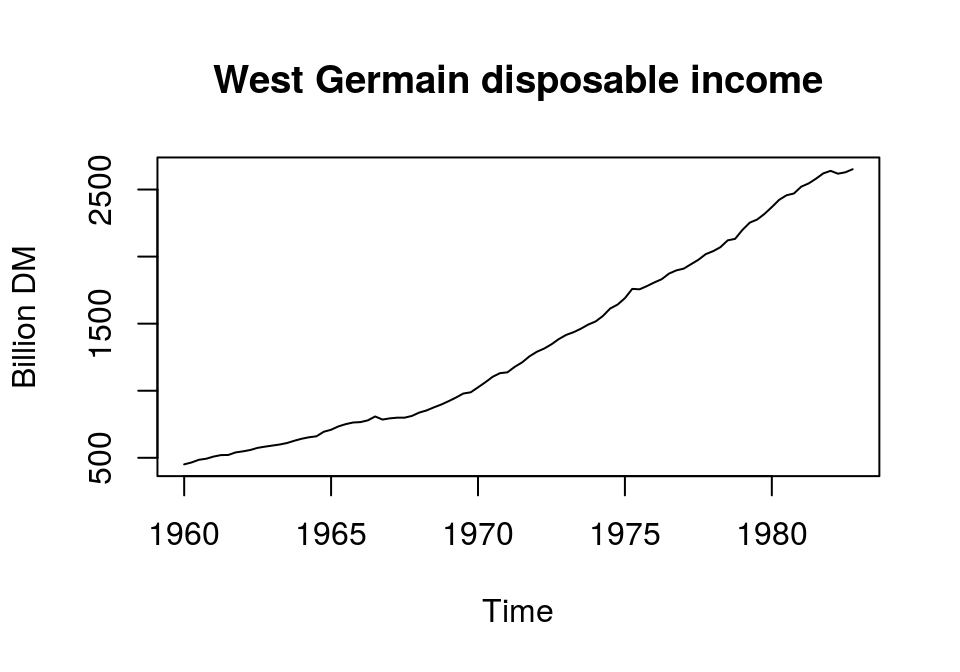
The series is continuously increasing and, thus, does not fluctuate around a constant mean. Furthermore, if we calculated the variances for an increasing window of periods from the beginning of the series to the end, we would see a constant increase in the estimated values. Therefore, disposable income in levels does not seem to be a stationary series. But how can we make this series stationary? For this it is useful to know that there are two popular models for nonstationary series, trend- and difference-stationary models.1
Trend-stationary: A series is trend-stationary, if it fluctuates around a deterministic trend, to which it reverts in the long run. Subtracting this trend from the original series yields a stationary series. For example, assuming that log disposable income follows a linear trend, we can regress the series on a constant and a linear trend and use the residuals as a candidate for a stationary series:
# Obtain ln of income
lincome <- log(income)

# Obtain detrended series
t_lincome <- (lincome - fitted(lm(lincome ~ I(1:length(lincome))))) * 100

# Plot and add horizontal line at 0
plot(t_lincome, main = "West German Disposable Income",
     ylab = "Deviation from linear trend"); abline(h = 0)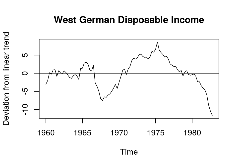
Although the mean of the resulting series is (practially) zero, its variance could be considered to increase over time. This might be due to the assumption of a simple linear trend. In this case we could search for better ways to extract the trend from this series, for example by adding a squared trend or by useing more sophisticated routines. However, note that the results of any time series analysis with trend stationary data might be sensitive to the method that was chosen to estimated the trend component of the series. It is very important to keep this in mind.
Apart from refining the method for estimating the deterministic trend of the series, the strong deviation of the actual values from the linear trend and its smoothness could also indicate a unit root, which would be associated with a difference stationary process.
Difference-stationary: If a time series can be made stationary by differencing, it is said to contain a unit root. In essence, this means that the current value of a series \(y_t\) is equal to its last value \(y_{t - 1}\) plus an error \(\epsilon_t\), i.e. \(y_t = a y_{t - 1} + \epsilon_t\) with \(|a| = 1\). Variables that show this behaviour are also said to be integrated of order d, or \(I\)(d), which means that d differences are neccesary to render a series stationary. According to the Box-Jenking approach - which is associated with ARIMA models - most economic time series can be made stationary by differencing the log of the series. Usually, one or two differencing operations should be enough.
Note that a time series can still contain a unit root, even when a deterministic trend was already removed. So, differencing the detrended series might still be necessary to render a series stationary.
In the case of the time series of disposable income it appears that the series is stationary after calculating the first differences of the natural logarithm. It flucuates around a relatively constant mean, exhibits a rather constant variance and is more erratic as the detrended series.2
# Obtain first log-differences of disposable income
d_lincome <- diff(log(e1[,"income"])) * 100

# # Plot and add horizontal line at 0
plot(d_lincome, main = "West German disposable income",
     ylab = "Log growth rate"); abline(h = 0)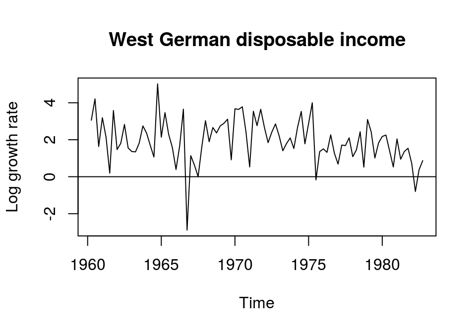
By looking at the results above, it seems that disposable income is difference-stationary with \(I\)(1). But since these are rather subjective impressions, more formal tests should be applied to check this.
Tests
Correlogram
When working with the Box-Jenkins approach it is common to check the stationarity of a time series by visual inspection of the correlogram, i.e. a plot containing the \(k\)th-order normalised autocorrelations. If the estimated autocorrelations die out rather quickly, the series is likely to be stationary.
In the following example, the autocorrelation function (ACF) is obtained for log disposable income in levels. Since the estimated autocorrelations remain above the confidence interval for all periods, the series is rather not stationary…
lincome <- log(income)
plot(lincome, main = "Log income...", ylab = NA)
acf(lincome, main = "...and corresponding ACF", ylab = NA)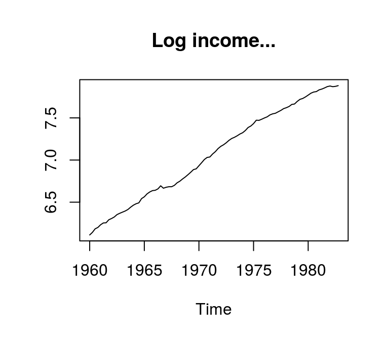
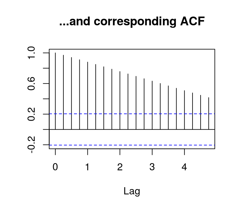
…and the detrended series shows similar features.
plot(t_lincome, main = "Deviation from linear trend...", ylab = NA)
acf(t_lincome, main = "...and corresponding ACF", ylab = NA)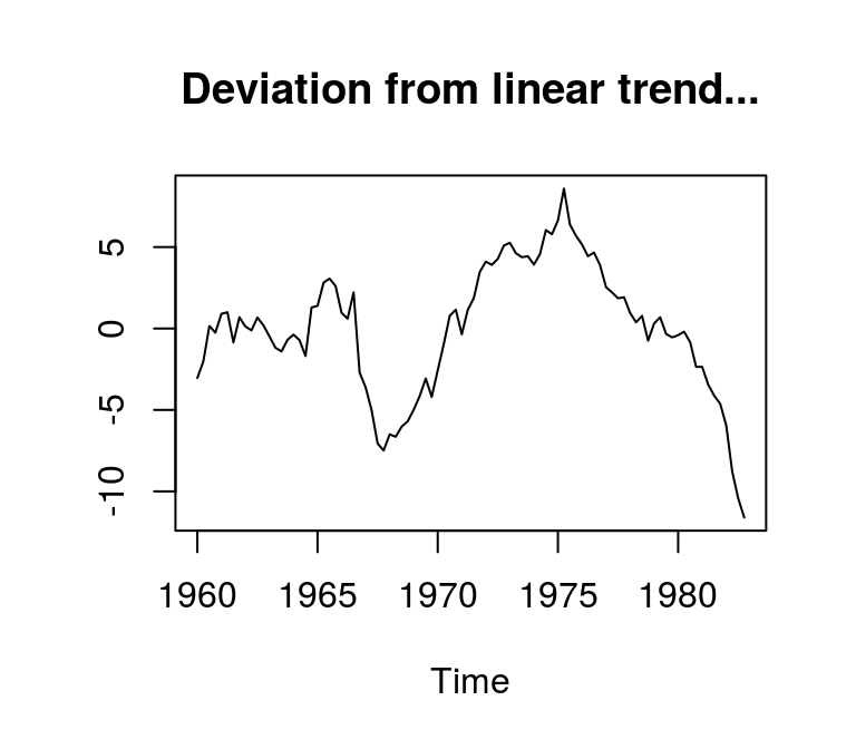
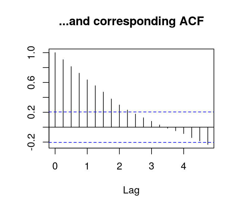
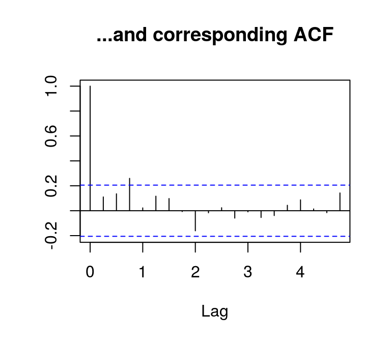
By contrast, the autocorrelations of the differenced log series die out rather quickly, which indicates stationarity.
plot(d_lincome, main = "First difference of log income...", ylab = NA)
acf(d_lincome, main = "...and corresponding ACF", ylab = NA)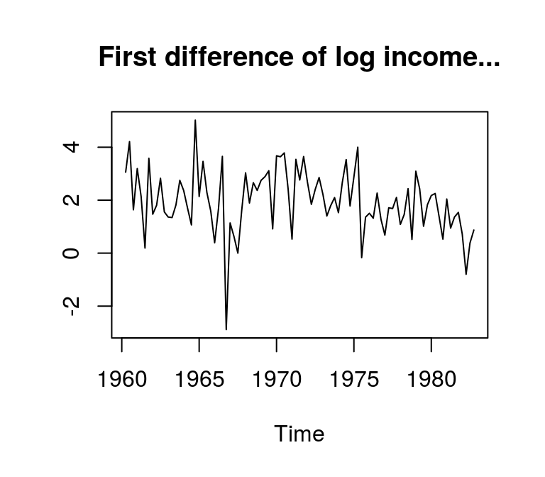
Unit root tests
Unit root tests help in assessing whether a time series is stationary. Due to the statistical issues that are associated with \(I\)(1) series, this is a very difficult task. Therefore, there is series of unit root tests and proposals under which circumstances a test is more useful than another. In the following some popular tests are presented.
For all tests the same data on log levels as well as first and second log differences are used. All series have the same length.
d1_lincome <- diff(lincome) # First difference
d2_lincome <- diff(d1_lincome) # Second difference

# Combine
data <- cbind(lincome, d1_lincome, d2_lincome)

# Get rid of NAs so that all have same length
data <- na.omit(data)

# Rename columsn
dimnames(data)[[2]] <- c("level", "diff_1", "diff_2")
The tseries package contains the unit root tests that are used here.
library(tseries)Augmented Dickey-Fuller test
The augmented Dickey-Fuller (ADF) test (Said and Dickey, 1984) seems to be the most popular unit root test. It estimates the equation
\[\Delta y_t = \mu + \beta t + (\theta - 1) y_{t - 1} + \sum \delta_i \Delta y_{t - i} + \epsilon_t,\]
where \(\theta\) is the variable of interest. The null hypothesis of the ADF test is that the series contains a unit root. If \(\theta\) is significantly different from 1, this would indicate stationarity. In the following code the ADF test is performed for a series of lag orders.
adf <- data.frame(k = 0:9,
                  level = NA,
                  diff_1 = NA,
                  diff_2 = NA)

# Run test for a series fo models
for (i in 1:nrow(adf)) {
  k <- adf$k[i]
  pos <- (9 - k + 1):nrow(data) # Position of used observations
  for (j in c("level", "diff_1", "diff_2")) {
    adf_test <- adf.test(data[pos, j], alternative = "stationary", k = k)
    adf[i, j] <- adf_test$p.value
  }
}

# Show results
adf
## k level diff_1 diff_2
## 1 0 0.9900000 0.01000000 0.01000000
## 2 1 0.9900000 0.01000000 0.01000000
## 3 2 0.9900000 0.06318328 0.01000000
## 4 3 0.9659595 0.19862916 0.01000000
## 5 4 0.9570174 0.36135454 0.01000000
## 6 5 0.9390069 0.45127002 0.01000000
## 7 6 0.9249955 0.46563987 0.03763891
## 8 7 0.9334218 0.16353566 0.03603800
## 9 8 0.9888206 0.21500947 0.01178816
## 10 9 0.9900000 0.41652671 0.01000000The results show that the null of a unit root cannot be rejected for all lags of the series in levels. For the first differenced series the picture is mixed. For lower lag orders, the test rejects the null, but not for higher lags. For the series with data in second differences the results clearly suggest a unit root.
The original Dickey-Fuller (DF) test has proven to be not very useful in practise. Therefore, it is not covered here.
KPSS
In contrast to many other unit root tests the null hypothesis of the KPSS test (Kwiatkowski et al., 1992) is that an observable time series is (trend-)stationary. Function kpss.test allows to specify a null, where the series is level stationary or trend stationary. Since the log-series shows clear signs of a linear trend, argument null is set to "Trend" for the variable in levels. For the first and second differences the argument is set to "Level".
kpss <- data.frame(level = NA,
                   diff_1 = NA,
                   diff_2 = NA)

# Run test for level data
kpss[, "level"] <- kpss.test(data[pos, "level"], null = "Trend")$p.value

# Run test for first differences
kpss[, "diff_1"] <- kpss.test(data[pos, "diff_1"], null = "Level")$p.value

# Run test for second differences
kpss[, "diff_2"] <- kpss.test(data[pos, "diff_2"], null = "Level")$p.value

# Show results
kpss
## level diff_1 diff_2
## 1 0.01 0.07781436 0.1The results show that for log disposable income in levels the null of stationarity is rejected at a very high confidence level. However, the test fails to reject the null of stationariy for differenced data at the 5 percent level. This is further indication that log disposable income is \(I\)(1).
Literature
Hyndman, R., Athanasopoulos, G., Bergmeir, C., Caceres, G., Chhay, L., O’Hara-Wild, M., Petropoulos, F., Razbash, S., Wang, E., & Yasmeen, F. (2020). forecast: Forecasting functions for time series and linear models.
Kennedy, P. (2014). A guide to econometrics. Malden (Mass.): Blackwell Publishing 6th ed.
Kwiatkowski, D., Phillips, P. C. B., Schmidt, P., & Shin, Y. (1992): Testing the null hypothesis of stationarity against the alternative of a unit root. Journal of Econometrics 54, 159–178.
Luetkepohl, H. (2007). New introduction to multiple time series analyis. Berlin: Springer.
Said, S. E., & Dickey, D. A. (1984). Testing for unit roots in autoregressive-moving average models of unknown order. Biometrika 71(3), 599–607.
A slightly more technical summary of difference and trend stationary processes can be found on mathworks.com.↩
In case you wondered, the first difference of the detrended series of disposable income looks exactly like the differenced log-series, except that it has a different mean.↩