Can a Bayesian VAR Beat Professional Forecasters?
with tags r bvartools bvar var bayes forecasting austria macroeconomicsA comparison between the models one happens to have written down answers a narrow question: which of them fits and forecasts best. It does not answer whether any of them is worth using. The benchmark for that is the forecast somebody actually published and was held to. This post runs that comparison for Austria, where three Bayesian VAR models compete against the projections of the European Commission, the ECB, the IHS, the IMF, the Austrian central bank and WIFO – and against the simplest competitor of them all, which is to carry the last observation forward.
The bvartools package has a function for exactly this. create_external_forecast turns published point forecasts into an object, which the rest of the estimation workflow treats as one more competitor: it can be combined with models, its forecast errors are calculated in the same call and it shows up as an extra column in the table of selection criteria. Everything below rests on it. If Bayesian VARs are new to you, the introduction to BVAR models is the better place to start.
Two data sets are needed and neither ships with the package, because bvartools does not depend on a particular source of data:
- The published projections come from the repository of macroeconomic projections, which collects the forecasts of public institutions in a machine-readable format. Forecasters are identified by their legal entity identifier (LEI), countries by the code of the IMF and variables by the conventions of the IMF’s World Economic Outlook. All forecasts in it are annual.
- The realised values come from EA-MD-QD (Barigozzi & Lissona, 2024), a collection of monthly and quarterly series for the euro area and its ten largest member countries, which is published as a set of Excel files on Zenodo.
library(bvartools)
library(readxl)
Realised values
EA-MD-QD is updated every month, so one release is pinned here – the one of August 2026 – which keeps the post reproducible. The DOI 10.5281/zenodo.10514667 always resolves to the most recent one. The archive contains one file per country, plus a copy of the raw data in a subfolder, which is not used here.
zip_url <- "https://zenodo.org/records/22233571/files/EA-MD-QD-2026-08.zip"
zip_file <- file.path(tempdir(), "ea-md-qd.zip")
download.file(zip_url, zip_file, mode = "wb", quiet = TRUE)

entries <- unzip(zip_file, list = TRUE)[["Name"]]
entry <- entries[basename(entries) == "ATdata.xlsx" & !grepl("/raw/", entries)]
unzip(zip_file, files = entry, exdir = tempdir(), junkpaths = TRUE)

raw <- as.data.frame(read_excel(file.path(tempdir(), "ATdata.xlsx"),
                                sheet = "data"))
The file is a monthly grid, in which quarterly series are only observed in the last month of a quarter. Since the published forecasts are annual, the three series that the forecasts can be matched to are aggregated to annual averages, and a year, for which not every period is observed, is dropped:
year <- as.integer(format(as.Date(raw[["Time"]]), "%Y"))

annual <- function(x, year, periods) {
  avail <- !is.na(x)
  value <- tapply(x[avail], year[avail], mean)
  value[tapply(x[avail], year[avail], length) == periods]
}

gdp <- annual(raw[["GDP_AT"]], year, 4)     # Real GDP, chain linked volumes
prc <- annual(raw[["HICPOV_AT"]], year, 12) # HICP, overall index
une <- annual(raw[["UNETOT_AT"]], year, 12) # Unemployment rate, total
The first two are levels and enter the model as annual rates of change, the third is already a rate. The columns carry the codes of the World Economic Outlook – NGDP_RPCH for real GDP growth, PCPIPCH for consumer price inflation and LUR for the unemployment rate – because create_external_forecast matches the published forecasts to the endogenous variables of a model by name.
years <- sort(as.integer(Reduce(intersect, list(names(gdp), names(prc),
                                                names(une)))))
pct <- function(x) {c(NA, 100 * (x[-1] / x[-length(x)] - 1))}

at <- ts(cbind(NGDP_RPCH = pct(gdp[as.character(years)]),
               PCPIPCH = pct(prc[as.character(years)]),
               LUR = as.numeric(une[as.character(years)])),
         start = min(years), frequency = 1)
at <- na.omit(at)

round(at, 1)
## Time Series:
## Start = 2001
## End = 2025
## Frequency = 1
## NGDP_RPCH PCPIPCH LUR
## 2001 1.2 2.9 4.0
## 2002 1.5 1.5 4.4
## 2003 1.1 1.3 4.8
## 2004 2.4 1.9 5.9
## 2005 2.4 2.1 6.0
## 2006 3.5 1.7 5.6
## 2007 3.7 2.2 5.2
## 2008 1.4 3.2 4.4
## 2009 -3.6 0.4 5.7
## 2010 1.7 1.7 5.2
## 2011 3.0 3.5 4.9
## 2012 0.7 2.6 5.2
## 2013 -0.3 2.1 5.7
## 2014 0.9 1.5 6.0
## 2015 1.3 0.8 6.2
## 2016 2.2 1.0 6.5
## 2017 2.4 2.2 5.9
## 2018 2.4 2.1 5.2
## 2019 1.7 1.5 4.8
## 2020 -6.4 1.4 6.1
## 2021 5.0 2.8 6.2
## 2022 5.4 8.6 4.7
## 2023 -0.7 7.7 5.1
## 2024 -0.8 2.9 5.2
## 2025 1.0 3.6 5.7plot(at, main = "")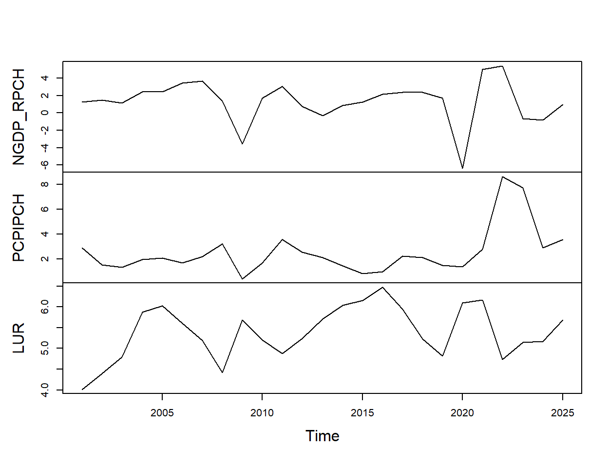
Twenty-five annual observations are not much for a VAR, which is the reason why the models below lean on their priors. The sample also contains the two episodes that decide most of this comparison: the collapse of 2020 and the inflation of 2022.
Published forecasts
The forecasts are a single file in long format with one point forecast per row. It is filtered to Austria, whose code is 122, and to the three variables of the model. Six institutions publish for Austria and are given their usual abbreviation here, because the LEI is not readable and the full name is long:
fcst <- read.csv(paste0("https://github.com/franzmohr/macroprojections/",
                        "raw/master/data/forecasts.csv"))

institutions <- c("254900ZNYA1FLUQ9U393" = "EC",
                  "549300DTUYXVMJXZNY75" = "ECB",
                  "529900FMFN29HKS4BE19" = "IHS",
                  "E7EXN6FJGRUTJYNZ3Z71" = "IMF",
                  "5299001Z8JOKGWV5O949" = "OeNB",
                  "5299004QA39L2ORLX198" = "WIFO")

fcst <- fcst[as.character(fcst[["ctry"]]) == "122" &
               fcst[["variable"]] %in% colnames(at), ]
fcst[["institution"]] <- institutions[fcst[["institution"]]]
fcst <- fcst[!is.na(fcst[["institution"]]), ]

head(fcst[order(fcst[["pubdate"]]), ], 3)
## year ctry variable pubdate value institution
## 3110 2001 122 LUR 2001-12-01 3.8 ECB
## 3111 2002 122 LUR 2001-12-01 3.9 ECB
## 3112 2003 122 LUR 2001-12-01 3.8 ECBThe names behind the abbreviations come with the data:
inst_names <- read.csv(paste0("https://github.com/franzmohr/macroprojections/",
                              "raw/master/data/institutions.csv"))
inst_names <- inst_names[match(names(institutions),
                               inst_names[["institution"]]), ]

cat(paste0(format(institutions, width = 5),
           inst_names[["institution_name"]]), sep = "\n")
## EC European Commission
## ECB European Central Bank
## IHS Institut für Höhere Studien - Institute for Advanced Studies (IHS)
## IMF International Monetary Fund
## OeNB Oesterreichische Nationalbank
## WIFO Österreichisches Institut für WirtschaftsforschungHow far back a forecaster can be followed differs a lot. The ECB publishes twice a year since 2001, while the others enter the data set around 2020:
pubdates <- lapply(split(fcst[["pubdate"]], fcst[["institution"]]), unique)

data.frame(Publications = lengths(pubdates),
           First = sapply(pubdates, min),
           Last = sapply(pubdates, max))
## Publications First Last
## EC 13 2021-11-11 2025-11-17
## ECB 49 2001-12-01 2025-12-01
## IHS 25 2020-06-26 2026-04-10
## IMF 10 2021-04-06 2025-10-14
## OeNB 21 2020-05-28 2026-03-24
## WIFO 26 2019-12-19 2026-04-10This is why the comparison below is run twice. The first race uses the long history of a single institution, the second one accepts a short sample in exchange for a crowded field. Pooling both would compare forecasters on different periods, and a period is by far the largest influence on how hard a forecast is.
The competitors
All models are estimated with an expanding window, so that each of them produces a sequence of forecasts from a training sample that grows by one year at a time. The following function runs the workflow:
iterations <- 10000
burnin <- 2000

estimate <- function(object, start, n_ahead) {
  object <- use_expanding_window(object, start = start)
  object <- add_initial_values(object)
  object <- add_posterior_coefficients(object)
  object <- add_posterior_loglik(object)
  object <- add_forecast_input(object, n_ahead = n_ahead)
  add_posterior_forecasts(object)
}
Three specifications enter the race: a VAR(1) with a plain, weakly informative prior, a VAR(2) with a Minnesota prior and a VAR(2) with stochastic search variable selection. They are produced by a function as well, because both races draw on them:
specifications <- function(data) {

  var_1 <- create_bvarmodel(data, p = 1, deterministic = "const",
                            iterations = iterations, burnin = burnin)
  var_1 <- add_priors(var_1,
                      coef = list(v_i = 1 / 10, v_i_det = 1 / 100),
                      sigma = list(df = 3, scale = 1))

  var_2 <- create_bvarmodel(data, p = 2, deterministic = "const",
                            iterations = iterations, burnin = burnin)
  var_2 <- add_priors(var_2,
                      coef = list(minnesota = list(kappa1 = 0.5, kappa2 = 0.5,
                                                   kappa4 = 5)),
                      sigma = list(df = 3, scale = 1))

  var_3 <- create_bvarmodel(data, p = 2, deterministic = "const",
                            varsel = "ssvs",
                            iterations = iterations, burnin = burnin)
  var_3 <- add_priors(var_3,
                      coef = list(v_i = 1 / 10, v_i_det = 1 / 100),
                      sigma = list(df = 3, scale = 1),
                      varsel = list(inprior = 0.5, tau = c(0.05, 10),
                                    exclude_deterministic = TRUE))

  list("BVAR(1)" = var_1, "BVAR(2), Minnesota" = var_2,
       "BVAR(2), SSVS" = var_3)
}
Relative forecast errors need a reference and a model is a poor one, because it is the thing under examination. The usual reference is the forecast that carries the last observation forward. It is a point forecast like the published ones, so create_external_forecast accepts it in the same way. The function below writes it in the long format that the function expects, where origin is the period, in which a forecast is published, and period the one it is made for:
no_change <- function(data, start, n_ahead) {

  ends <- seq(start - 1, end(data)[1])
  result <- expand.grid(end = ends, h = 1:n_ahead, variable = colnames(data),
                        KEEP.OUT.ATTRS = FALSE, stringsAsFactors = FALSE)

  # The last observation of a training sample, carried forward
  rows <- match(result[["end"]], as.numeric(time(data)))
  cols <- match(result[["variable"]], colnames(data))
  result[["value"]] <- as.matrix(data)[cbind(rows, cols)]

  # A publication one year after the end of a training sample is matched to
  # that sample, which is what 'data_lag = 1' states below
  result[["origin"]] <- result[["end"]] + 1
  result[["period"]] <- result[["end"]] + result[["h"]]

  result[!is.na(result[["value"]]), ]
}
The long race
The first race covers the forecasts for 2013 to 2025 and pits the three models and the no-change benchmark against the ECB, the only forecaster with publications throughout that period. Forecasts are made three years ahead.
The estimation window starts in 2013 because the shortest training sample has to support the largest model. With the first forecast period set to 2013 the models are estimated on twelve observations to begin with, which a VAR(2) in three variables still survives. An earlier start makes the residual covariance of the first window singular.
set.seed(7788)

start_1 <- 2013
specs <- specifications(at)
models_1 <- lapply(specs, estimate, start = start_1, n_ahead = 3)
The no-change benchmark is built from the same data:
rw_1 <- create_external_forecast(no_change(at, start_1, n_ahead = 3),
                                 models_1[[1]], data_lag = 1)
For the ECB the columns of the data have to be named, since they do not follow the defaults of the function. data_lag = 1 states that the annual figures of a year are only available in the course of the following one, so that a forecast published in 2021 is matched to the training sample which ends in 2020. Its projection for 2021 is then the one-year ahead forecast of the institution and of the models alike. select = "first" keeps the earliest publication, if several are matched to the same training sample: the ECB projects in June and in December, and the June projection is the one that knows less about the year it forecasts.
ecb <- create_external_forecast(fcst[fcst[["institution"]] == "ECB", ],
                                models_1[[1]],
                                period = "year", origin = "pubdate",
                                variable = "variable", value = "value",
                                data_lag = 1, select = "first")

ecb
## External forecasts
##
## Variables: NGDP_RPCH, PCPIPCH, LUR
## Forecast horizon: 3
## Publications: 13
##
## Publication Training sample ends
## 2013.414 2012
## 2014.414 2013
## 2015.414 2014
## 2016.415 2015
## 2017.414 2016
## 2018.414 2017
## 2019.414 2018
## 2020.415 2019
## 2021.414 2020
## 2022.414 2021
## 2023.414 2022
## 2024.415 2023
## 2025.414 2024Thirteen publications are matched to thirteen training samples, which is one per window. From here on the external forecasts follow the workflow of the models:
race_1 <- combine_models(models_1[[1]], models_1[[2]], models_1[[3]],
                         rw_1, ecb)
race_1 <- add_forecast_errors(race_1, test_sample = at)

sc_1 <- selection_criteria(race_1)
The printed comparison numbers the competitors in the order, in which they were combined:
data.frame(Model = paste("Model", 1:length(race_1)),
           Competitor = c(names(specs), "No change", "ECB"))
## Model Competitor
## 1 Model 1 BVAR(1)
## 2 Model 2 BVAR(2), Minnesota
## 3 Model 3 BVAR(2), SSVS
## 4 Model 4 No change
## 5 Model 5 ECBErrors are shown relative to the no-change benchmark, so an entry below one means that a competitor beats it and the two columns can be read against each other:
print(sc_1, relative = 4)##
## ------------------------------------------
## In-sample
## ------------------------------------------
##
## Log-likelihood
##
## Mean Median Quantile (2.5%) Quantile (97.5%)
## Model 1 -111.5 -111.2 -118.8 -106.21
## Model 2 -103.7 -103.5 -112.0 -96.95
## Model 3 -102.7 -102.0 -113.4 -95.77
## Model 4 NA NA NA NA
## Model 5 NA NA NA NA
##
##
## Akaike Information Criterion (AIC)
##
## Mean Median Quantile (2.5%) Quantile (97.5%)
## Model 1 259.1 258.4 248.4 273.7
## Model 2 261.4 260.9 247.9 277.9
## Model 3 259.4 257.9 245.5 280.8
## Model 4 NA NA NA NA
## Model 5 NA NA NA NA
##
##
## Bayesian Information Criterion (BIC)
##
## Mean Median Quantile (2.5%) Quantile (97.5%)
## Model 1 280.3 279.6 269.6 294.9
## Model 2 292.1 291.6 278.5 308.6
## Model 3 290.1 288.6 276.2 311.5
## Model 4 NA NA NA NA
## Model 5 NA NA NA NA
##
##
## Hannan-Quinn Criterion (HQ)
##
## Mean Median Quantile (2.5%) Quantile (97.5%)
## Model 1 264.7 264.0 254.1 279.3
## Model 2 269.1 268.6 255.6 285.7
## Model 3 267.1 265.6 253.3 288.6
## Model 4 NA NA NA NA
## Model 5 NA NA NA NA
##
##
## ------------------------------------------
## Out-of-sample
## ------------------------------------------
##
## Mean absolute forecast errors (MAFE)
##
## Variable h Model 1 Model 2 Model 3 Model 4 Model 5
## NGDP_RPCH 1 1.2803 1.0751 1.1973 1 0.3150
## PCPIPCH 1 1.3426 1.3491 1.3271 1 0.3545
## LUR 1 1.5129 1.4790 1.4600 1 0.9137
## NGDP_RPCH 2 0.9095 0.8415 0.8504 1 0.4415
## PCPIPCH 2 0.8559 0.8555 0.8168 1 0.6183
## LUR 2 1.1353 1.1763 1.0056 1 0.6700
## NGDP_RPCH 3 0.9847 0.9508 0.9064 1 0.6026
## PCPIPCH 3 0.9783 0.9690 0.9163 1 0.7094
## LUR 3 1.3569 1.4372 1.1053 1 1.1913
##
##
## Root mean squared forecast errors (RMSFE)
##
## Variable h Model 1 Model 2 Model 3 Model 4 Model 5
## NGDP_RPCH 1 0.8988 0.8158 0.8694 1 0.2001
## PCPIPCH 1 1.2005 1.1623 1.1871 1 0.3484
## LUR 1 1.5002 1.4546 1.4152 1 0.8640
## NGDP_RPCH 2 0.8163 0.7624 0.7722 1 0.5140
## PCPIPCH 2 0.9119 0.9179 0.8963 1 0.7285
## LUR 2 1.3298 1.3520 1.1430 1 0.7769
## NGDP_RPCH 3 1.0387 0.9936 0.9409 1 0.7182
## PCPIPCH 3 0.9746 0.9448 0.9173 1 0.8492
## LUR 3 1.5800 1.5932 1.2170 1 1.1147The in-sample criteria are empty for the last two competitors. Neither is estimated, so there is no likelihood to evaluate, and the same applies to the credible bands of the out-of-sample statistics, which are degenerate for a point forecast.
Three things stand out. The ECB wins almost everywhere and at the one-year horizon it wins by a distance: its root mean squared error for GDP growth is a fifth of the no-change benchmark and a quarter of the best model. The models lose that horizon to the benchmark in absolute errors for all three variables, and only in squared errors, and only for GDP growth, are they ahead of it – carrying the last figure forward is usually the closer forecast but occasionally a catastrophic one, and the two statistics weigh that differently. Finally, the lead of the ECB narrows as the horizon grows. At three years it stands at 0.60 against 0.91 for GDP growth and at 0.71 against 0.92 for inflation, and for the unemployment rate the model with variable selection has the smaller absolute error of the two, with both of them behind the benchmark.
plot(sc_1, criterion = "AFE")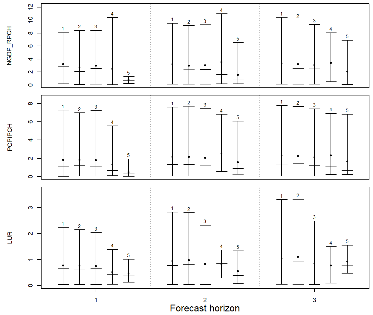
Where the difference comes from is easier to see period by period. The following plot repeats the comparison for the first model, the benchmark and the ECB, which keeps it readable:
duel <- combine_models(models_1[[1]], rw_1, ecb)
duel <- add_forecast_errors(duel, test_sample = at)
plot_forecast_errors_by_period(duel, criterion = "AFE")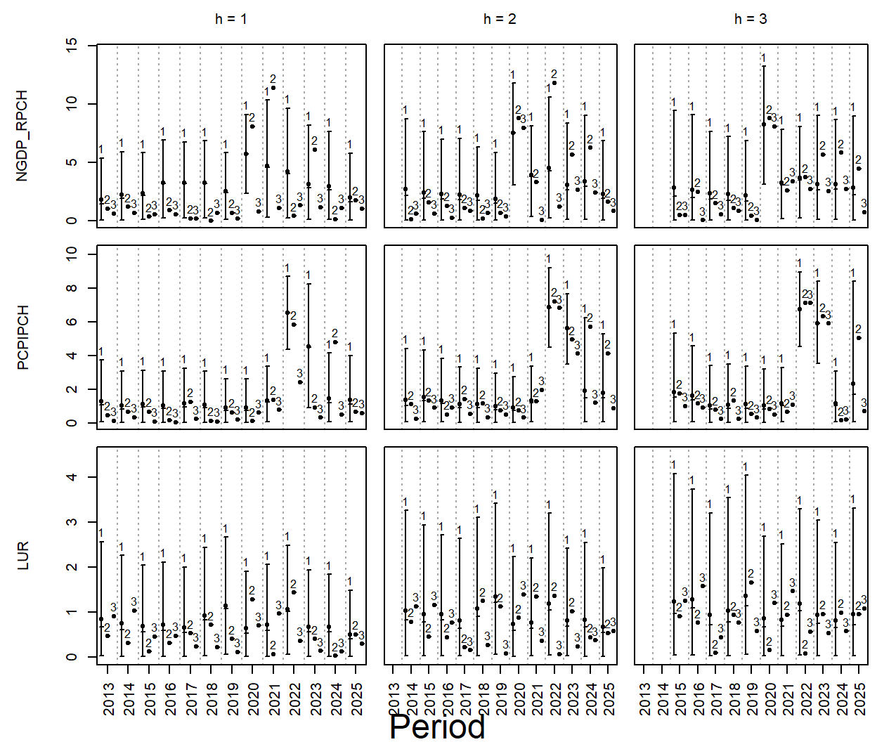
In the quiet years between 2013 and 2019 the three competitors are hard to tell apart. The gap is made in 2020, 2022 and 2023, when the model misses the collapse of output and the inflation that followed it by several percentage points, while the ECB, forecasting in June of the respective year, misses them by much less. That is less a statement about models than about information sets, which the closing section returns to.
The crowded race
The second race adds the five remaining institutions. All of them publish from 2021 on, so the estimation window starts there, which leaves six training samples and forecasts for 2021 to 2025. Since not every institution projects three years ahead, the horizon is cut to two, which keeps the field comparable. Of the models only the one with stochastic search variable selection is carried over, because the three specifications were close to each other in the first race and eight competitors are as many as the printed table holds:
start_2 <- 2021
model_2 <- estimate(specs[["BVAR(2), SSVS"]], start = start_2, n_ahead = 2)

rw_2 <- create_external_forecast(no_change(at, start_2, n_ahead = 2),
                                 model_2, data_lag = 1)
Argument by produces one object per forecaster, which is returned as a list of class modellist and can be handed to combine_models as a whole:
pros <- create_external_forecast(fcst[fcst[["pubdate"]] >= "2021-01-01", ],
                                 model_2,
                                 period = "year", origin = "pubdate",
                                 variable = "variable", value = "value",
                                 by = "institution", data_lag = 1,
                                 select = "first")

names(pros)
## [1] "EC" "OeNB" "WIFO" "IHS" "ECB" "IMF"race_2 <- combine_models(model_2, rw_2, pros)
race_2 <- add_forecast_errors(race_2, test_sample = at)
sc_2 <- selection_criteria(race_2)
data.frame(Model = paste("Model", 1:length(race_2)),
Competitor = c("BVAR(2), SSVS", "No change", names(pros)))## Model Competitor
## 1 Model 1 BVAR(2), SSVS
## 2 Model 2 No change
## 3 Model 3 EC
## 4 Model 4 OeNB
## 5 Model 5 WIFO
## 6 Model 6 IHS
## 7 Model 7 ECB
## 8 Model 8 IMFprint(sc_2, relative = 2)##
## ------------------------------------------
## In-sample
## ------------------------------------------
##
## Log-likelihood
##
## Mean Median Quantile (2.5%) Quantile (97.5%)
## Model 1 -103.6 -102.8 -114.6 -95.92
## Model 2 NA NA NA NA
## Model 3 NA NA NA NA
## Model 4 NA NA NA NA
## Model 5 NA NA NA NA
## Model 6 NA NA NA NA
## Model 7 NA NA NA NA
## Model 8 NA NA NA NA
##
##
## Akaike Information Criterion (AIC)
##
## Mean Median Quantile (2.5%) Quantile (97.5%)
## Model 1 261.1 259.7 245.8 283.2
## Model 2 NA NA NA NA
## Model 3 NA NA NA NA
## Model 4 NA NA NA NA
## Model 5 NA NA NA NA
## Model 6 NA NA NA NA
## Model 7 NA NA NA NA
## Model 8 NA NA NA NA
##
##
## Bayesian Information Criterion (BIC)
##
## Mean Median Quantile (2.5%) Quantile (97.5%)
## Model 1 291.8 290.3 276.5 313.8
## Model 2 NA NA NA NA
## Model 3 NA NA NA NA
## Model 4 NA NA NA NA
## Model 5 NA NA NA NA
## Model 6 NA NA NA NA
## Model 7 NA NA NA NA
## Model 8 NA NA NA NA
##
##
## Hannan-Quinn Criterion (HQ)
##
## Mean Median Quantile (2.5%) Quantile (97.5%)
## Model 1 268.9 267.4 253.6 290.9
## Model 2 NA NA NA NA
## Model 3 NA NA NA NA
## Model 4 NA NA NA NA
## Model 5 NA NA NA NA
## Model 6 NA NA NA NA
## Model 7 NA NA NA NA
## Model 8 NA NA NA NA
##
##
## ------------------------------------------
## Out-of-sample
## ------------------------------------------
##
## Mean absolute forecast errors (MAFE)
##
## Variable h Model 1 Model 2 Model 3 Model 4 Model 5 Model 6 Model 7 Model 8
## NGDP_RPCH 1 0.8026 1 0.2820 0.3323 0.3777 0.3978 0.2924 0.4017
## PCPIPCH 1 1.1288 1 0.6074 0.4014 0.4529 0.3941 0.3359 0.4430
## LUR 1 1.4354 1 1.5816 1.1310 1.0136 0.7279 0.7736 0.6771
## NGDP_RPCH 2 0.4992 1 0.2434 0.2947 0.3262 0.2710 0.2828 0.3011
## PCPIPCH 2 0.7407 1 0.5860 0.6223 0.5951 0.6223 0.5905 0.5998
## LUR 2 0.9338 1 0.1580 0.2617 0.4346 0.4346 0.3753 0.4971
##
##
## Root mean squared forecast errors (RMSFE)
##
## Variable h Model 1 Model 2 Model 3 Model 4 Model 5 Model 6 Model 7 Model 8
## NGDP_RPCH 1 0.6663 1 0.1976 0.2327 0.2791 0.2829 0.1996 0.2947
## PCPIPCH 1 1.1252 1 0.7184 0.4215 0.4230 0.4299 0.3433 0.4430
## LUR 1 1.2508 1 1.2317 0.9799 0.8597 0.6269 0.6925 0.5543
## NGDP_RPCH 2 0.5406 1 0.2587 0.2812 0.3008 0.2685 0.2675 0.3028
## PCPIPCH 2 0.8636 1 0.7371 0.7542 0.7360 0.7744 0.7207 0.7821
## LUR 2 1.1077 1 0.1445 0.2918 0.4646 0.4062 0.3995 0.4728plot(sc_2, criterion = "AFE")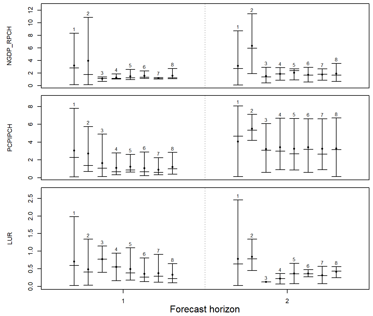
The six institutions are close to each other and clearly ahead of the model for output and for prices, which is the same picture as in the long race and the one that the literature on forecast comparisons usually reports. The unemployment rate is the exception. At the one-year horizon the no-change benchmark beats the model and three of the six institutions, and only at two years is the whole field ahead of it: the annual Austrian unemployment rate moves slowly, and carrying the last figure forward is a strong forecast of it. Five forecast periods are far too few to read more than an order of magnitude out of these numbers.
What this comparison does and does not show
A model that loses such a race has not been shown to be a bad model, and it is worth being precise about what separates the two sides.
The information sets differ. This is the main one. An institution publishing in June knows the quarterly national accounts and the monthly price and labour market figures of the year it forecasts, while the annual model knows nothing about that year at all. At the one-year horizon the institutions are therefore doing something closer to nowcasting than to forecasting, which is exactly where their lead is largest, and it narrows as the horizon grows. Choosing select = "first" and an annual data_lag narrows the gap but does not close it. A model that is to be compared on equal terms would have to be estimated on quarterly or monthly data and its forecasts aggregated to years.
The realisations are revised. The institutions forecast the figures as they stood at the time, and are scored here against the data as they stand today. The models are estimated on those revised data as well, which in this respect works in their favour: they are fitted to a history that the forecasters did not have. A comparison free of this objection needs real-time vintages on both sides.
The definitions are not identical. In the conventions of the World Economic Outlook, PCPIPCH is national consumer price inflation, whereas the realisation used here is the HICP, and NGDP_RPCH is headline annual growth, whereas the realisation is aggregated from seasonally and calendar adjusted quarters. Both differences are small for Austria but they are not zero, and part of what is measured as a forecast error is really a difference in definition.
Point forecasts are compared. The models produce a predictive distribution and only its centre enters these statistics. Whatever a Bayesian VAR contributes beyond a point forecast – the credible bands, the probability of a contraction – has no counterpart in the published projections and is not rewarded here.
The samples are short. Thirteen forecast periods in the long race and five in the crowded one, both dominated by the same two unusual years. Mean errors from samples of this size are indicative, not conclusive.
References
Barigozzi, M., & Lissona, C. (2024). Large datasets for the Euro Area and its member countries and the dynamic effects of the common monetary policy. arXiv:2410.05082. https://doi.org/10.48550/arXiv.2410.05082
Barigozzi, M., & Lissona, C. (2026). EA-MD-QD: Large Euro Area and Euro Member Countries Datasets for Macroeconomic Research (Version 08.2026) [Data set]. Zenodo. https://doi.org/10.5281/zenodo.10514667
Chan, J., Koop, G., Poirier, D. J., & Tobias, J. L. (2019). Bayesian Econometric Methods (2nd ed.). Cambridge: University Press.
George, E. I., Sun, D., & Ni, S. (2008). Bayesian stochastic search for VAR model restrictions. Journal of Econometrics, 142(1), 553-580. https://doi.org/10.1016/j.jeconom.2007.08.017
Litterman, R. B. (1986). Forecasting with Bayesian vector autoregressions – five years of experience. Journal of Business & Economic Statistics, 4(1), 25-38. https://doi.org/10.2307/1391384
